Quickstart
Here is a quick rundown of ffn’s capabilities. For a more complete guide, read the source, or check out the API docs.
import ffn
%matplotlib inline
Data Retrieval
The main method for data retrieval is the get function. The get function uses a data provider to download data from an external service and packs that data into a pandas DataFrame for further manipulation.
Note: Upon import,
ffnmodifiespandas.core.base.PandasObjectto provide added functionality to pandas objects, including DataFrames.
data = ffn.get('agg,hyg,spy,eem,efa', start='2010-01-01', end='2014-01-01')
print(data.head())
                  agg        hyg        spy        eem        efa
Date
2010-01-04  74.942818  43.466671  89.225403  33.181232  38.846069
2010-01-05  75.283783  43.672871  89.461578  33.422070  38.880318
2010-01-06  75.240242  43.785816  89.524582  33.491989  39.044666
2010-01-07  75.153183  43.962566  89.902481  33.297764  38.894009
2010-01-08  75.196701  44.031300  90.201675  33.561905  39.202148
By default, the data is downloaded from Yahoo! Finance and the Adjusted Close is used as the security’s price. Other data sources are also available and you may select other fields as well. Fields are specified by using the following format: {ticker}:{field}. So, if we want to get the Open, High, Low, Close for aapl, we would do the following:
print(ffn.get('aapl:Open,aapl:High,aapl:Low,aapl:Close', start='2010-01-01', end='2014-01-01').head())
            aaplopen  aaplhigh   aapllow  aaplclose
Date
2010-01-04  7.622500  7.660714  7.585000   7.643214
2010-01-05  7.664286  7.699643  7.616071   7.656429
2010-01-06  7.656429  7.686786  7.526786   7.534643
2010-01-07  7.562500  7.571429  7.466071   7.520714
2010-01-08  7.510714  7.571429  7.466429   7.570714
The default data provider is ffn.data.web(). This is basically just a thin wrapper around pandas’ pandas.io.data provider. Please refer to the appropriate docs for more info (data sources, etc.). The ffn.data.csv() provider is also available when we want to load data from a local file. In this case, we can tell ffn.data.get() to use the csv provider. In this case, we also want to merge this new data with the existing data we downloaded earlier. Therefore, we will provide the data object as the existing argument, and the new data will be merged into the existing DataFrame.
data = ffn.get('dbc', provider=ffn.data.csv, path='test_data.csv', existing=data)
print(data.head())
                  agg        hyg        spy        eem        efa    dbc
Date
2010-01-04  74.942818  43.466671  89.225403  33.181232  38.846069  25.24
2010-01-05  75.283783  43.672871  89.461578  33.422070  38.880318  25.27
2010-01-06  75.240242  43.785816  89.524582  33.491989  39.044666  25.72
2010-01-07  75.153183  43.962566  89.902481  33.297764  38.894009  25.40
2010-01-08  75.196701  44.031300  90.201675  33.561905  39.202148  25.38
As we can see above, the dbc column was added to the DataFrame. Internally, get is using the function ffn.merge, which is useful when you want to merge TimeSeries and DataFrames together. We plan on adding many more data sources over time. If you know your way with Python and would like to contribute a data provider, please feel free to submit a pull request - contributions are always welcome!
Data Manipulation
Now that we have some data, let’s start manipulating it. In quantitative finance, we are often interested in the returns of a given time series. Let’s calculate the returns by simply calling the to_returns or to_log_returns extension methods.
returns = data.to_log_returns().dropna()
print(returns.head())
                 agg       hyg       spy       eem       efa       dbc
Date
2010-01-05  0.004539  0.004733  0.002643  0.007232  0.000881  0.001188
2010-01-06 -0.000579  0.002583  0.000704  0.002090  0.004218  0.017651
2010-01-07 -0.001158  0.004029  0.004212 -0.005816 -0.003866 -0.012520
2010-01-08  0.000579  0.001562  0.003322  0.007901  0.007891 -0.000788
2010-01-11 -0.000772 -0.000893  0.001395 -0.002085  0.008176 -0.003157
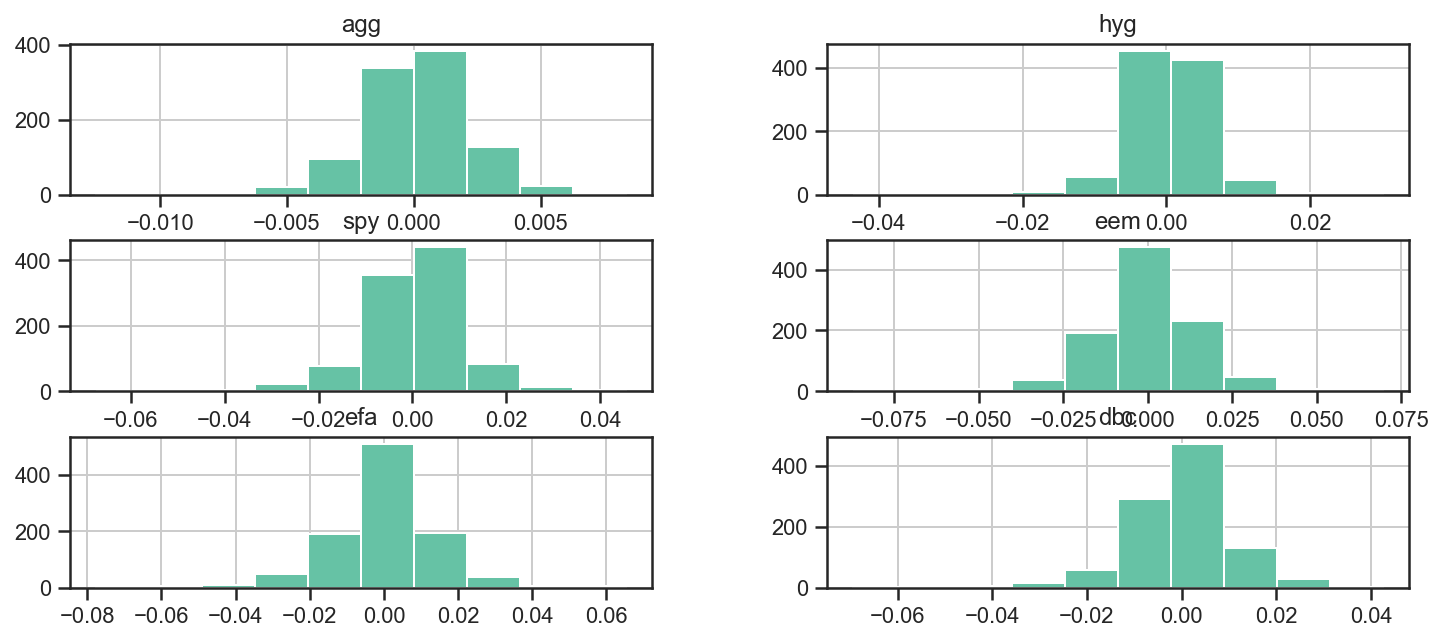
Let’s look at the different distributions to see how they look.
ax = returns.hist(figsize=(12, 5))
We can also use the numerous functions packed into numpy, pandas and the like to further analyze the returns. For example, we can use the corr function to get the pairwise correlations between assets.
returns.corr().as_format('.2f')
| agg | hyg | spy | eem | efa | dbc | |
|---|---|---|---|---|---|---|
| agg | 1.00 | -0.12 | -0.33 | -0.23 | -0.29 | -0.18 |
| hyg | -0.12 | 1.00 | 0.77 | 0.75 | 0.76 | 0.49 |
| spy | -0.33 | 0.77 | 1.00 | 0.88 | 0.92 | 0.59 |
| eem | -0.23 | 0.75 | 0.88 | 1.00 | 0.90 | 0.62 |
| efa | -0.29 | 0.76 | 0.92 | 0.90 | 1.00 | 0.61 |
| dbc | -0.18 | 0.49 | 0.59 | 0.62 | 0.61 | 1.00 |
Here we used the convenience method as_format to have a prettier output. We could also plot a heatmap to better visualize the results.
returns.plot_corr_heatmap();
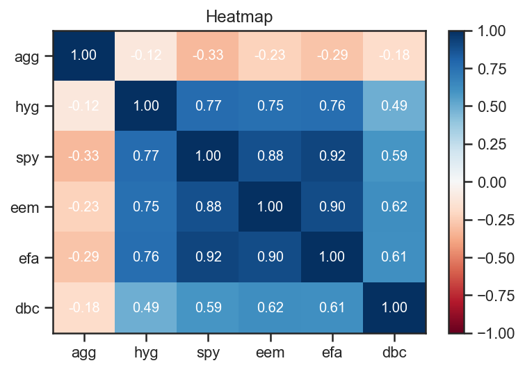
We used the ffn.core.plot_corr_heatmap(), which is a convenience method that simply calls ffn’s ffn.core.plot_heatmap() with sane arguments.
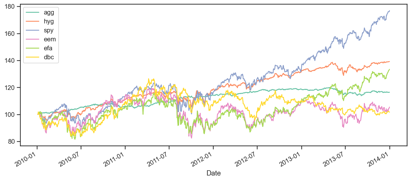
Let’s start looking at how all these securities performed over the period. To achieve this, we will plot rebased time series so that we can see how they each performed relative to each other.
ax = data.rebase().plot(figsize=(12,5))
Performance Measurement
For a more complete view of each asset’s performance over the period, we can use the ffn.core.calc_stats() method which will create a ffn.core.GroupStats object. A GroupStats object wraps a bunch of ffn.core.PerformanceStats objects in a dict with some added convenience methods.
perf = data.calc_stats()
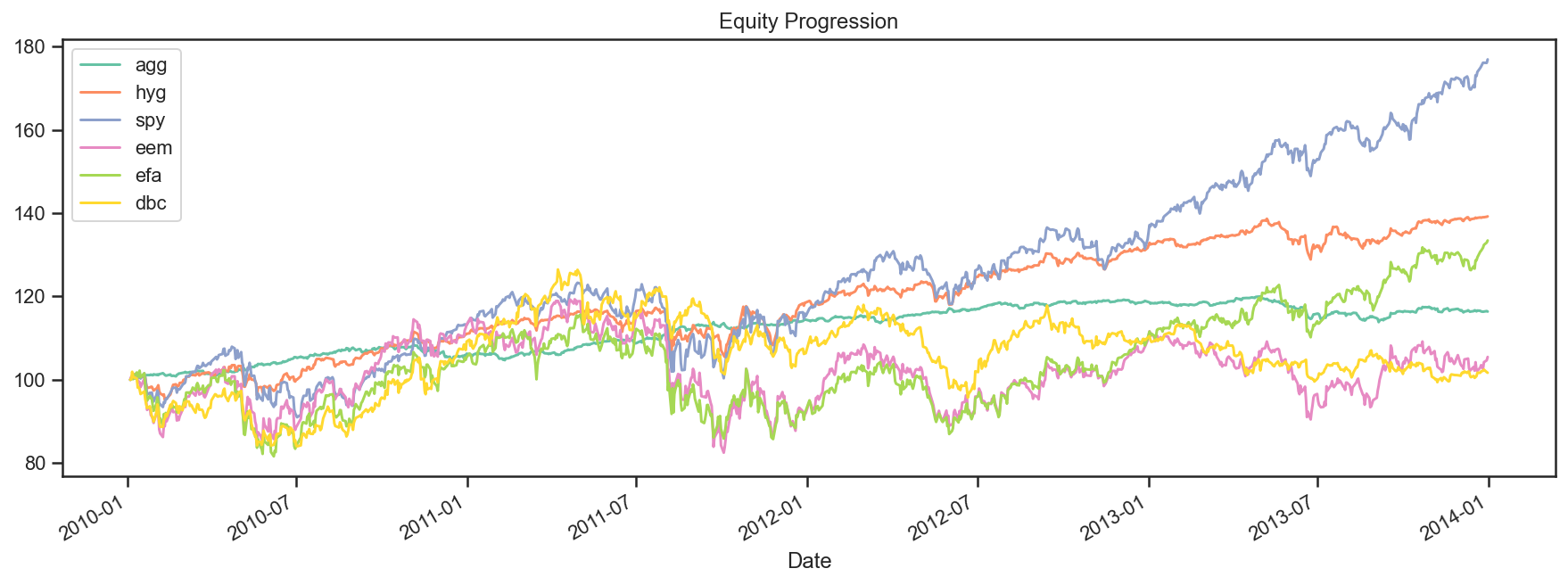
Now that we have our GroupStats object, we can analyze the performance in greater detail. For example, the plot method yields a graph similar to the one above.
perf.plot();
We can also display a wide array of statistics that are all contained in the PerformanceStats object. This will probably look crappy in the docs, but do try it out in a Notebook. We are also actively trying to improve the way we display this wide array of stats.
print(perf.display())
Stat                 agg         hyg         spy         eem         efa         dbc
-------------------  ----------  ----------  ----------  ----------  ----------  ----------
Start                2010-01-04  2010-01-04  2010-01-04  2010-01-04  2010-01-04  2010-01-04
End                  2013-12-31  2013-12-31  2013-12-31  2013-12-31  2013-12-31  2013-12-31
Risk-free rate       0.00%       0.00%       0.00%       0.00%       0.00%       0.00%

Total Return         16.36%      39.22%      76.92%      5.46%       33.43%      1.66%
Daily Sharpe         1.11        0.97        0.93        0.18        0.44        0.11
Daily Sortino        1.84        1.51        1.48        0.29        0.69        0.17
CAGR                 3.87%       8.65%       15.37%      1.34%       7.50%       0.41%
Max Drawdown         -5.14%      -10.06%     -18.61%     -30.87%     -25.86%     -24.34%
Calmar Ratio         0.75        0.86        0.83        0.04        0.29        0.02

MTD                  -0.56%      0.41%       2.59%       -0.41%      2.18%       0.59%
3m                   0.02%       3.42%       10.52%      3.48%       6.08%       -0.39%
6m                   0.57%       5.84%       16.32%      9.55%       18.12%      2.11%
YTD                  -1.98%      5.75%       32.31%      -3.65%      21.44%      -7.63%
1Y                   -1.98%      5.75%       32.31%      -3.65%      21.44%      -7.63%
3Y (ann.)            3.08%       7.83%       16.07%      -2.34%      8.17%       -2.34%
5Y (ann.)            -           -           -           -           -           -
10Y (ann.)           -           -           -           -           -           -
Since Incep. (ann.)  3.87%       8.65%       15.37%      1.34%       7.50%       0.41%

Daily Sharpe         1.11        0.97        0.93        0.18        0.44        0.11
Daily Sortino        1.84        1.51        1.48        0.29        0.69        0.17
Daily Mean (ann.)    3.86%       8.70%       15.73%      4.35%       9.73%       1.83%
Daily Vol (ann.)     3.48%       8.97%       16.83%      24.56%      22.31%      16.84%
Daily Skew           -0.40       -0.55       -0.39       -0.12       -0.26       -0.47
Daily Kurt           2.30        7.50        4.03        3.06        3.64        2.90
Best Day             0.84%       3.05%       4.65%       7.20%       6.74%       4.34%
Worst Day            -1.24%      -4.26%      -6.51%      -8.34%      -7.46%      -6.70%

Monthly Sharpe       1.23        1.11        1.22        0.30        0.60        0.27
Monthly Sortino      2.49        2.19        2.36        0.53        1.06        0.43
Monthly Mean (ann.)  3.59%       9.51%       16.99%      6.43%       11.06%      4.61%
Monthly Vol (ann.)   2.93%       8.56%       13.91%      21.45%      18.41%      17.10%
Monthly Skew         -0.34       0.14        -0.32       -0.10       -0.37       -0.74
Monthly Kurt         0.02        1.75        0.24        1.28        0.17        1.16
Best Month           1.77%       8.49%       10.91%      16.27%      11.61%      9.89%
Worst Month          -2.00%      -5.30%      -7.95%      -17.89%     -11.19%     -14.62%

Yearly Sharpe        0.65        2.79        1.10        -0.06       0.50        -0.40
Yearly Sortino       2.77        inf         inf         -0.11       1.32        -0.58
Yearly Mean          3.16%       7.85%       16.73%      -1.13%      9.32%       -2.24%
Yearly Vol           4.86%       2.82%       15.22%      19.05%      18.72%      5.57%
Yearly Skew          -0.54       1.49        0.22        0.58        -1.69       0.27
Yearly Kurt          -           -           -           -           -           -
Best Year            7.70%       11.06%      32.31%      19.05%      21.44%      3.50%
Worst Year           -1.98%      5.75%       1.89%       -18.79%     -12.23%     -7.63%

Avg. Drawdown        -0.48%      -1.18%      -1.78%      -5.16%      -4.96%      -5.09%
Avg. Drawdown Days   16.95       15.70       17.55       78.22       60.04       107.85
Avg. Up Month        0.83%       1.86%       3.58%       5.87%       4.37%       4.28%
Avg. Down Month      -0.49%      -2.31%      -3.21%      -3.41%      -4.15%      -3.35%
Win Year %           66.67%      100.00%     100.00%     33.33%      66.67%      33.33%
Win 12m %            81.08%      97.30%      94.59%      59.46%      70.27%      45.95%
None
Lots to look at here. We can also access the underlying PerformanceStats for each series, either by index or name.
# we can also use perf[2] in this case
perf['spy'].display_monthly_returns()
  Year    Jan    Feb    Mar    Apr    May    Jun    Jul    Aug    Sep    Oct    Nov    Dec    YTD
------  -----  -----  -----  -----  -----  -----  -----  -----  -----  -----  -----  -----  -----
  2010  -5.24   3.12   6.09   1.55  -7.95  -5.17   6.83  -4.5    8.96   3.82   0      6.69  13.14
  2011   2.33   3.47   0.01   2.9   -1.12  -1.69  -2     -5.5   -6.94  10.91  -0.41   1.04   1.89
  2012   4.64   4.34   3.22  -0.67  -6.01   4.06   1.18   2.51   2.54  -1.82   0.57   0.89  15.99
  2013   5.12   1.28   3.8    1.92   2.36  -1.33   5.17  -3      3.16   4.63   2.96   2.59  32.31
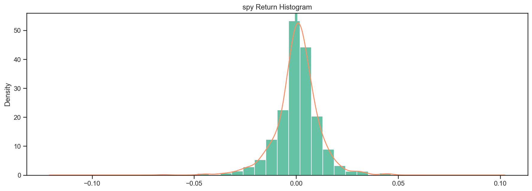
perf[2].plot_histogram();
Most of the stats are also available as pandas objects - see the stats, return_table, lookback_returns attributes.
perf['spy'].stats
start                    2010-01-04 00:00:00
end                      2013-12-31 00:00:00
rf                                       0.0
total_return                        0.769155
cagr                                 0.15375
max_drawdown                       -0.186055
calmar                              0.826367
mtd                                 0.025926
three_month                         0.105247
six_month                           0.163183
ytd                                 0.323077
one_year                            0.323077
three_year                           0.16066
five_year                                NaN
ten_year                                 NaN
incep                                0.15375
daily_sharpe                         0.93439
daily_sortino                       1.478916
daily_mean                          0.157279
daily_vol                           0.168323
daily_skew                         -0.388777
daily_kurt                          4.028481
best_day                            0.046499
worst_day                          -0.065123
monthly_sharpe                      1.221065
monthly_sortino                     2.362922
monthly_mean                        0.169906
monthly_vol                         0.139146
monthly_skew                       -0.319921
monthly_kurt                        0.235707
best_month                          0.109147
worst_month                        -0.079455
yearly_sharpe                       1.099284
yearly_sortino                           inf
yearly_mean                          0.16731
yearly_vol                          0.152199
yearly_skew                          0.21847
yearly_kurt                              NaN
best_year                           0.323077
worst_year                           0.01895
avg_drawdown                       -0.017845
avg_drawdown_days                  17.550725
avg_up_month                        0.035827
avg_down_month                     -0.032066
win_year_perc                            1.0
twelve_month_win_perc               0.945946
dtype: object
Numerical Routines and Financial Functions
ffn also provides commonly used numerical routines and plans to add many more in the future. One can easily determine the proper weights using a mean-variance approach using the ffn.core.calc_mean_var_weights() function.
returns.calc_mean_var_weights().as_format('.2%')
agg    79.52%
hyg     6.47%
spy    14.01%
eem     0.00%
efa     0.00%
dbc     0.00%
dtype: object
Some other interesting functions are the clustering routines, such as a Python implementation of David Varadi’s Fast Threshold Clustering Algorithm (FTCA)
returns.calc_ftca(threshold=0.8)
{1: ['eem', 'spy', 'efa'], 2: ['agg'], 3: ['dbc'], 4: ['hyg']}