Examples
Here are a few examples to give you a better idea of what bt is all about.
SMA Strategy
Let’s start off with a Simple Moving Average (SMA) strategy. We will start with a simple version of the strategy, namely:
Select the securities that are currently above their 50 day moving average
Weigh each selected security equally
Rebalance the portfolio to reflect the target weights
This should be pretty simple to build. The only thing missing above is the calculation of the simple moving average. When should this take place?
Given the flexibility of bt, there is no strict rule. The average calculation could be performed in an Algo, but that would be pretty inefficient. A better way would be to calculate the moving average at the beginning - before starting the backtest. After all, all the data is known in advance.
Now that we know what we have to do, let’s get started. First we will download some data and calculate the simple moving average.
import bt
%matplotlib inline
# download data
data = bt.get('aapl,msft,c,gs,ge', start='2010-01-01')

# calculate moving average DataFrame using pandas' rolling_mean
import pandas as pd
# a rolling mean is a moving average, right?
sma = data.rolling(50).mean()
It’s always a good idea to plot your data to make sure it looks ok. So let’s see how the data + sma plot looks like.
# let's see what the data looks like - this is by no means a pretty chart, but it does the job
plot = bt.merge(data, sma).plot(figsize=(15, 5))
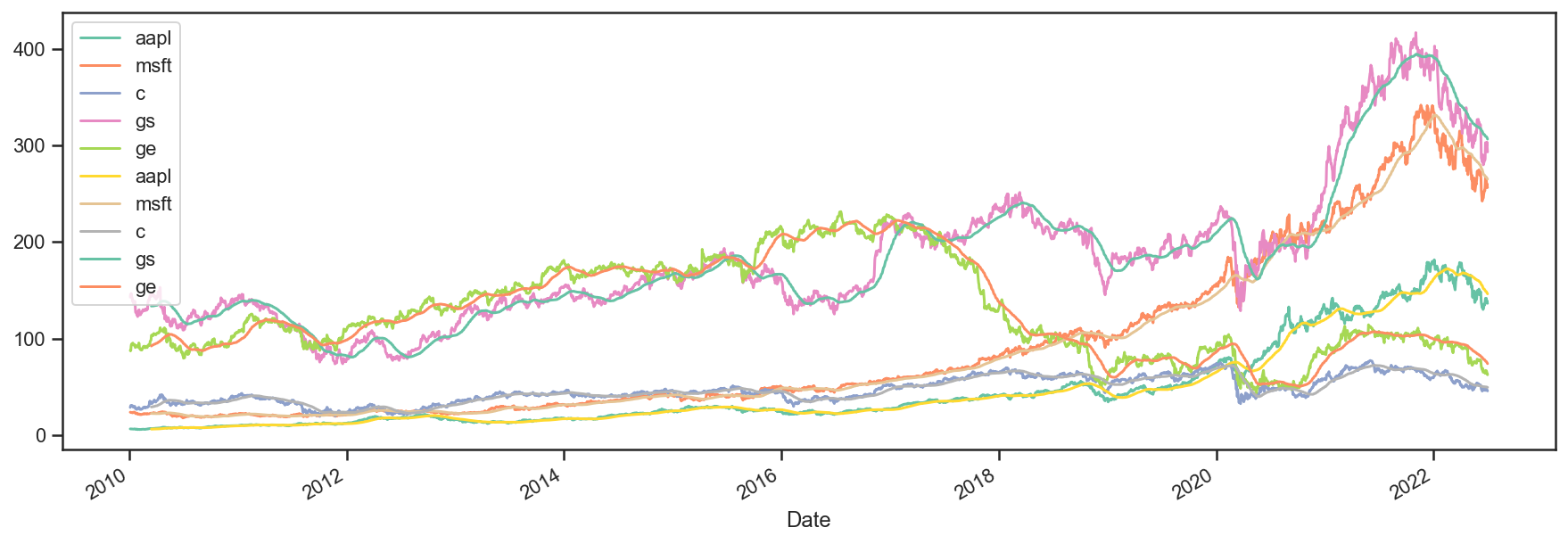
Looks legit.
Now that we have our data, we will need to create our security selection logic. Let’s create a basic Algo that will select the securities that are above their moving average.
Before we do that, let’s think about how we will code it. We could pass the SMA data and then extract the row (from the sma DataFrame) on the current date, compare the values to the current prices, and then keep a list of those securities where the price is above the SMA. This is the most straightforward approach. However, this is not very re-usable because the logic within the Algo will be quite specific to the task at hand and if we wish to change the logic, we will have to write a new algo.
For example, what if we wanted to select securities that were below their sma? Or what if we only wanted securities that were 5% above their sma?
What we could do instead is pre-calculate the selection logic DataFrame (a fast, vectorized operation) and write a generic Algo that takes in this boolean DataFrame and returns the securities where the value is True on a given date. This will be must faster and much more reusable. Let’s see how the implementation looks like.
class SelectWhere(bt.Algo):

    """
    Selects securities based on an indicator DataFrame.

    Selects securities where the value is True on the current date (target.now).

    Args:
        * signal (DataFrame): DataFrame containing the signal (boolean DataFrame)

    Sets:
        * selected

    """
    def __init__(self, signal):
        self.signal = signal

    def __call__(self, target):
        # get signal on target.now
        if target.now in self.signal.index:
            sig = self.signal.loc[target.now]

            # get indices where true as list
            selected = list(sig.index[sig])

            # save in temp - this will be used by the weighing algo
            target.temp['selected'] = selected

        # return True because we want to keep on moving down the stack
        return True
So there we have it. Our selection Algo.
Note
By the way, this Algo already exists - I just wanted to show you how you would code it from scratch.
Here is the code.
All we have to do now is pass in a signal matrix. In our case, it’s quite easy:
signal = data > sma
Simple, concise and more importantly, fast! Let’s move on and test the strategy.
# first we create the Strategy
s = bt.Strategy('above50sma', [SelectWhere(data > sma),
                               bt.algos.WeighEqually(),
                               bt.algos.Rebalance()])

# now we create the Backtest
t = bt.Backtest(s, data)

# and let's run it!
res = bt.run(t)
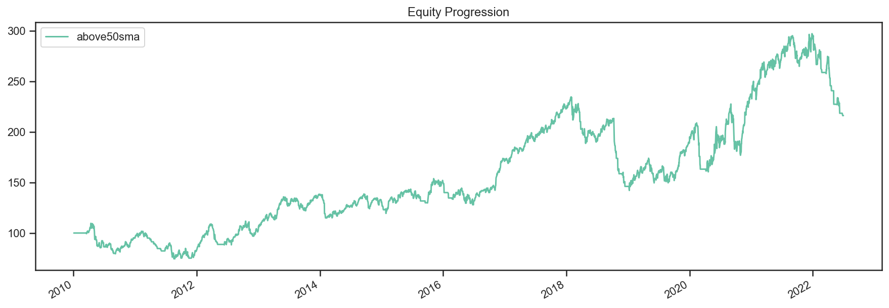
So just to recap, we created the strategy, created the backtest by joining Strategy+Data, and ran the backtest. Let’s see the results.
# what does the equity curve look like?
res.plot();
# and some performance stats
res.display()
 Stat                 above50sma
 -------------------  ------------
 Start                2010-01-03
 End                  2022-07-01
 Risk-free rate       0.00%

 Total Return         116.08%
 Daily Sharpe         0.42
 Daily Sortino        0.63
 CAGR                 6.36%
 Max Drawdown         -39.43%
 Calmar Ratio         0.16

 MTD                  0.00%
 3m                   -19.50%
 6m                   -26.03%
 YTD                  -26.03%
 1Y                   -22.10%
 3Y (ann.)            10.34%
 5Y (ann.)            1.89%
 10Y (ann.)           8.70%
 Since Incep. (ann.)  6.36%

 Daily Sharpe         0.42
 Daily Sortino        0.63
 Daily Mean (ann.)    8.07%
 Daily Vol (ann.)     19.45%
 Daily Skew           -0.65
 Daily Kurt           4.74
 Best Day             5.78%
 Worst Day            -8.26%

 Monthly Sharpe       0.39
 Monthly Sortino      0.65
 Monthly Mean (ann.)  8.59%
 Monthly Vol (ann.)   21.86%
 Monthly Skew         -0.37
 Monthly Kurt         0.73
 Best Month           21.65%
 Worst Month          -17.26%

 Yearly Sharpe        0.41
 Yearly Sortino       0.83
 Yearly Mean          9.78%
 Yearly Vol           23.65%
 Yearly Skew          -0.88
 Yearly Kurt          -0.67
 Best Year            34.85%
 Worst Year           -34.38%

 Avg. Drawdown        -3.56%
 Avg. Drawdown Days   47.27
 Avg. Up Month        4.76%
 Avg. Down Month      -5.35%
 Win Year %           66.67%
 Win 12m %            67.14%
Nothing stellar but at least you learnt something along the way (I hope).
Oh, and one more thing. If you were to write your own “library” of backtests, you might want to write yourself a helper function that would allow you to test different parameters and securities. That function might look something like this:
def above_sma(tickers, sma_per=50, start='2010-01-01', name='above_sma'):
    """
    Long securities that are above their n period
    Simple Moving Averages with equal weights.
    """
    # download data
    data = bt.get(tickers, start=start)
    # calc sma
    sma = data.rolling(sma_per).mean()

    # create strategy
    s = bt.Strategy(name, [SelectWhere(data > sma),
                           bt.algos.WeighEqually(),
                           bt.algos.Rebalance()])

    # now we create the backtest
    return bt.Backtest(s, data)
This function allows us to easily generate backtests. We could easily compare a few different SMA periods. Also, let’s see if we can beat a long-only allocation to the SPY.
# simple backtest to test long-only allocation
def long_only_ew(tickers, start='2010-01-01', name='long_only_ew'):
    s = bt.Strategy(name, [bt.algos.RunOnce(),
                           bt.algos.SelectAll(),
                           bt.algos.WeighEqually(),
                           bt.algos.Rebalance()])
    data = bt.get(tickers, start=start)
    return bt.Backtest(s, data)

# create the backtests
tickers = 'aapl,msft,c,gs,ge'
sma10 = above_sma(tickers, sma_per=10, name='sma10')
sma20 = above_sma(tickers, sma_per=20, name='sma20')
sma40 = above_sma(tickers, sma_per=40, name='sma40')
benchmark = long_only_ew('spy', name='spy')

# run all the backtests!
res2 = bt.run(sma10, sma20, sma40, benchmark)
res2.plot(freq='m');
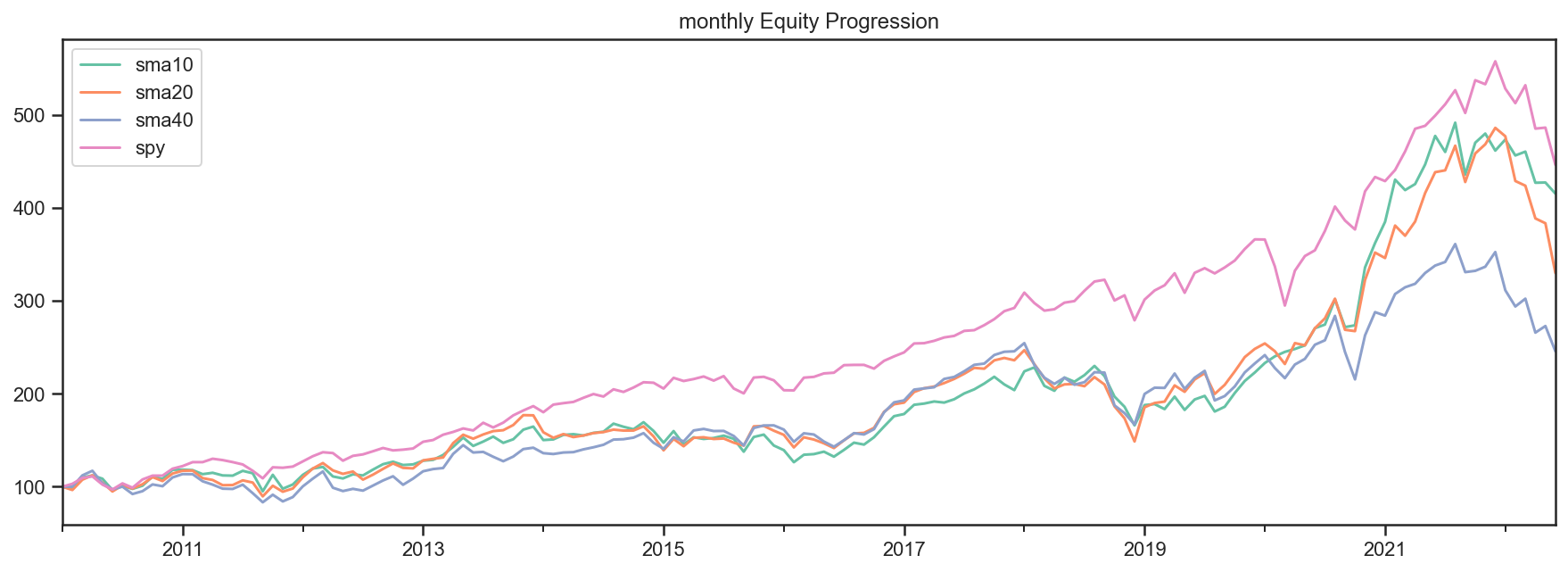
res2.display()
 Stat                 sma10       sma20       sma40       spy
 -------------------  ----------  ----------  ----------  ----------
 Start                2010-01-03  2010-01-03  2010-01-03  2010-01-03
 End                  2022-07-01  2022-07-01  2022-07-01  2022-07-01
 Risk-free rate       0.00%       0.00%       0.00%       0.00%

 Total Return         284.16%     229.80%     145.62%     321.22%
 Daily Sharpe         0.63        0.58        0.47        0.75
 Daily Sortino        0.99        0.91        0.73        1.15
 CAGR                 11.38%      10.03%      7.46%       12.20%
 Max Drawdown         -31.77%     -40.72%     -34.93%     -33.72%
 Calmar Ratio         0.36        0.25        0.21        0.36

 MTD                  -0.76%      0.00%       0.00%       -0.37%
 3m                   -10.58%     -22.25%     -18.82%     -16.66%
 6m                   -10.71%     -32.14%     -30.31%     -20.28%
 YTD                  -10.71%     -32.14%     -30.31%     -20.28%
 1Y                   -13.63%     -24.65%     -27.20%     -11.44%
 3Y (ann.)            28.10%      14.77%      3.73%       10.10%
 5Y (ann.)            15.80%      8.37%       1.96%       11.11%
 10Y (ann.)           13.76%      10.96%      9.67%       12.78%
 Since Incep. (ann.)  11.38%      10.03%      7.46%       12.20%

 Daily Sharpe         0.63        0.58        0.47        0.75
 Daily Sortino        0.99        0.91        0.73        1.15
 Daily Mean (ann.)    12.88%      11.52%      9.01%       13.03%
 Daily Vol (ann.)     20.48%      19.79%      18.97%      17.34%
 Daily Skew           -0.11       -0.29       -0.45       -0.59
 Daily Kurt           6.61        6.23        4.32        11.75
 Best Day             10.47%      10.47%      6.20%       9.06%
 Worst Day            -8.26%      -8.26%      -8.26%      -10.94%

 Monthly Sharpe       0.65        0.54        0.43        0.92
 Monthly Sortino      1.18        1.02        0.75        1.62
 Monthly Mean (ann.)  13.56%      11.95%      9.71%       13.00%
 Monthly Vol (ann.)   20.96%      21.94%      22.42%      14.20%
 Monthly Skew         -0.02       0.22        -0.10       -0.40
 Monthly Kurt         1.01        1.11        0.67        0.89
 Best Month           22.75%      24.73%      21.97%      12.70%
 Worst Month          -16.94%     -14.34%     -15.86%     -12.49%

 Yearly Sharpe        0.54        0.43        0.40        0.80
 Yearly Sortino       2.01        1.03        0.77        2.15
 Yearly Mean          13.38%      13.94%      9.76%       12.67%
 Yearly Vol           24.64%      32.80%      24.22%      15.79%
 Yearly Skew          0.41        -0.15       -0.87       -0.68
 Yearly Kurt          -0.43       -0.96       -0.59       0.12
 Best Year            62.47%      66.99%      39.35%      32.31%
 Worst Year           -18.59%     -37.01%     -32.06%     -20.28%

 Avg. Drawdown        -3.95%      -3.49%      -3.68%      -1.69%
 Avg. Drawdown Days   40.43       35.12       48.79       15.92
 Avg. Up Month        4.68%       5.00%       4.69%       3.20%
 Avg. Down Month      -5.00%      -4.85%      -5.70%      -3.56%
 Win Year %           58.33%      66.67%      75.00%      83.33%
 Win 12m %            68.57%      66.43%      69.29%      91.43%
And there you have it. Beating the market ain’t that easy!
SMA Crossover Strategy
Let’s build on the last section to test a moving average crossover strategy. The easiest way to achieve this is to build an Algo similar to SelectWhere, but for the purpose of setting target weights. Let’s call this algo WeighTarget. This algo will take a DataFrame of target weights that we will pre-calculate.
Basically, when the 50 day moving average will be above the 200-day moving average, we will be long (+1 target weight). Conversely, when the 50 is below the 200, we will be short (-1 target weight).
Here’s the WeighTarget implementation (this Algo also already exists in the algos module):
class WeighTarget(bt.Algo):
    """
    Sets target weights based on a target weight DataFrame.

    Args:
        * target_weights (DataFrame): DataFrame containing the target weights

    Sets:
        * weights

    """

    def __init__(self, target_weights):
        self.tw = target_weights

    def __call__(self, target):
        # get target weights on date target.now
        if target.now in self.tw.index:
            w = self.tw.loc[target.now]

            # save in temp - this will be used by the weighing algo
            # also dropping any na's just in case they pop up
            target.temp['weights'] = w.dropna()

        # return True because we want to keep on moving down the stack
        return True
So let’s start with a simple 50-200 day sma crossover for a single security.
## download some data & calc SMAs
data = bt.get('spy', start='2010-01-01')
sma50 = data.rolling(50).mean()
sma200 = data.rolling(200).mean()

## now we need to calculate our target weight DataFrame
# first we will copy the sma200 DataFrame since our weights will have the same strucutre
tw = sma200.copy()
# set appropriate target weights
tw[sma50 > sma200] = 1.0
tw[sma50 <= sma200] = -1.0
# here we will set the weight to 0 - this is because the sma200 needs 200 data points before
# calculating its first point. Therefore, it will start with a bunch of nulls (NaNs).
tw[sma200.isnull()] = 0.0
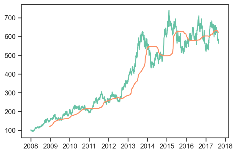
Ok so we downloaded our data, calculated the simple moving averages, and then we setup our target weight (tw) DataFrame. Let’s take a look at our target weights to see if they make any sense.
# plot the target weights + chart of price & SMAs
tmp = bt.merge(tw, data, sma50, sma200)
tmp.columns = ['tw', 'price', 'sma50', 'sma200']
ax = tmp.plot(figsize=(15,5), secondary_y=['tw'])
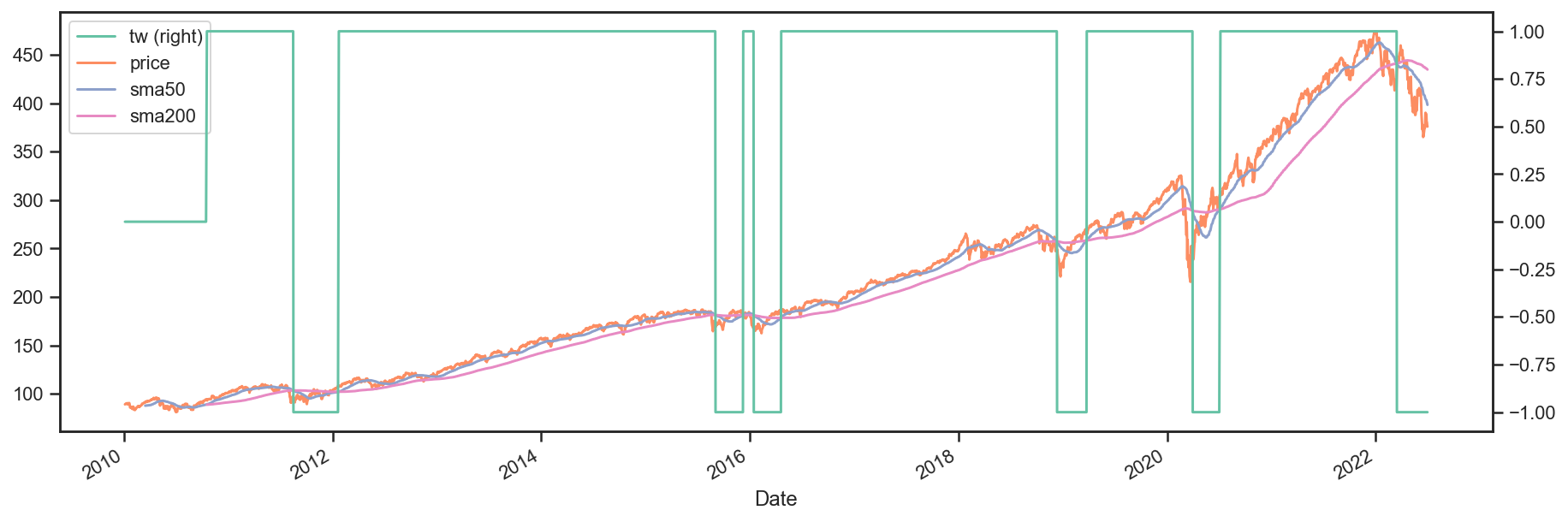
As mentioned earlier, it’s always a good idea to plot your strategy data. It is usually easier to spot logic/programming errors this way, especially when dealing with lots of data.
Now let’s move on with the Strategy & Backtest.
ma_cross = bt.Strategy('ma_cross', [WeighTarget(tw),
                                    bt.algos.Rebalance()])

t = bt.Backtest(ma_cross, data)
res = bt.run(t)
res.plot();
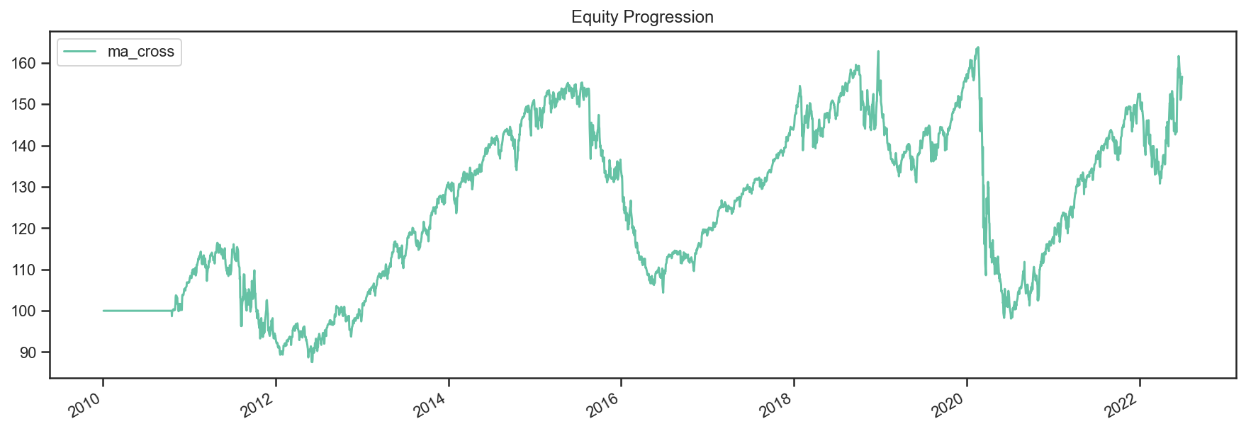
Ok great so there we have our basic moving average crossover strategy.
Exploring the Tree Structure
So far, we have explored strategies that allocate capital to securities. But what if we wanted to test a strategy that allocated capital to sub-strategies?
The most straightforward way would be to test the different sub-strategies, extract their equity curves and create “synthetic securities” that would basically just represent the returns achieved from allocating capital to the different sub-strategies.
Let’s see how this looks:
# first let's create a helper function to create a ma cross backtest
def ma_cross(ticker, start='2010-01-01',
             short_ma=50, long_ma=200, name='ma_cross'):
    # these are all the same steps as above
    data = bt.get(ticker, start=start)
    short_sma = data.rolling(short_ma).mean()
    long_sma  = data.rolling(long_ma).mean()

    # target weights
    tw = long_sma.copy()
    tw[short_sma > long_sma] = 1.0
    tw[short_sma <= long_sma] = -1.0
    tw[long_sma.isnull()] = 0.0

    # here we specify the children (3rd) arguemnt to make sure the strategy
    # has the proper universe. This is necessary in strategies of strategies
    s = bt.Strategy(name, [WeighTarget(tw), bt.algos.Rebalance()], [ticker])

    return bt.Backtest(s, data)

# ok now let's create a few backtests and gather the results.
# these will later become our "synthetic securities"
t1 = ma_cross('aapl', name='aapl_ma_cross')
t2 = ma_cross('msft', name='msft_ma_cross')

# let's run these strategies now
res = bt.run(t1, t2)

# now that we have run the strategies, let's extract
# the data to create "synthetic securities"
data = bt.merge(res['aapl_ma_cross'].prices, res['msft_ma_cross'].prices)

# now we have our new data. This data is basically the equity
# curves of both backtested strategies. Now we can just use this
# to test any old strategy, just like before.
s = bt.Strategy('s', [bt.algos.SelectAll(),
                      bt.algos.WeighInvVol(),
                      bt.algos.Rebalance()])

# create and run
t = bt.Backtest(s, data)
res = bt.run(t)
res.plot();

res.plot_weights();
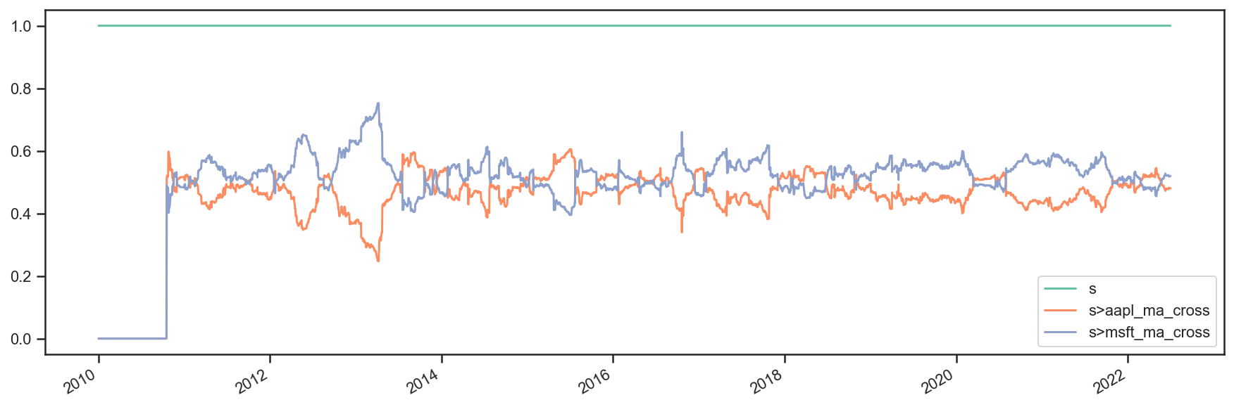
As we can see above, the process is a bit more involved, but it works. It is not very elegant though, and obtaining security-level allocation information is problematic.
Luckily, bt has built-in functionality for dealing with strategies of strategies. It uses the same general principal as demonstrated above but does it seamlessly. Basically, when a strategy is a child of another strategy, it will create a “paper trade” version of itself internally. As we run our strategy, it will run its internal “paper version” and use the returns from that strategy to populate the price property.
This means that the parent strategy can use the price information (which reflects the returns of the strategy had it been employed) to determine the appropriate allocation. Again, this is basically the same process as above, just packed into 1 step.
Perhaps some code will help:
# once again, we will create a few backtests
# these will be the child strategies
t1 = ma_cross('aapl', name='aapl_ma_cross')
t2 = ma_cross('msft', name='msft_ma_cross')

# let's extract the data object
data = bt.merge(t1.data, t2.data)

# now we create the parent strategy
# we specify the children to be the two
# strategies created above
s = bt.Strategy('s', [bt.algos.SelectAll(),
                      bt.algos.WeighInvVol(),
                      bt.algos.Rebalance()],
                [t1.strategy, t2.strategy])

# create and run
t = bt.Backtest(s, data)
res = bt.run(t)
res.plot();
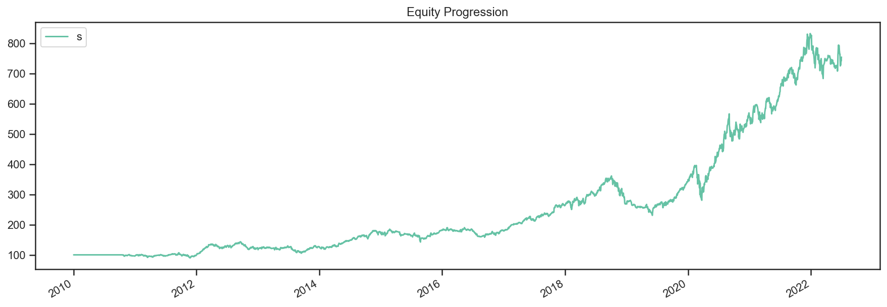
res.plot_weights();
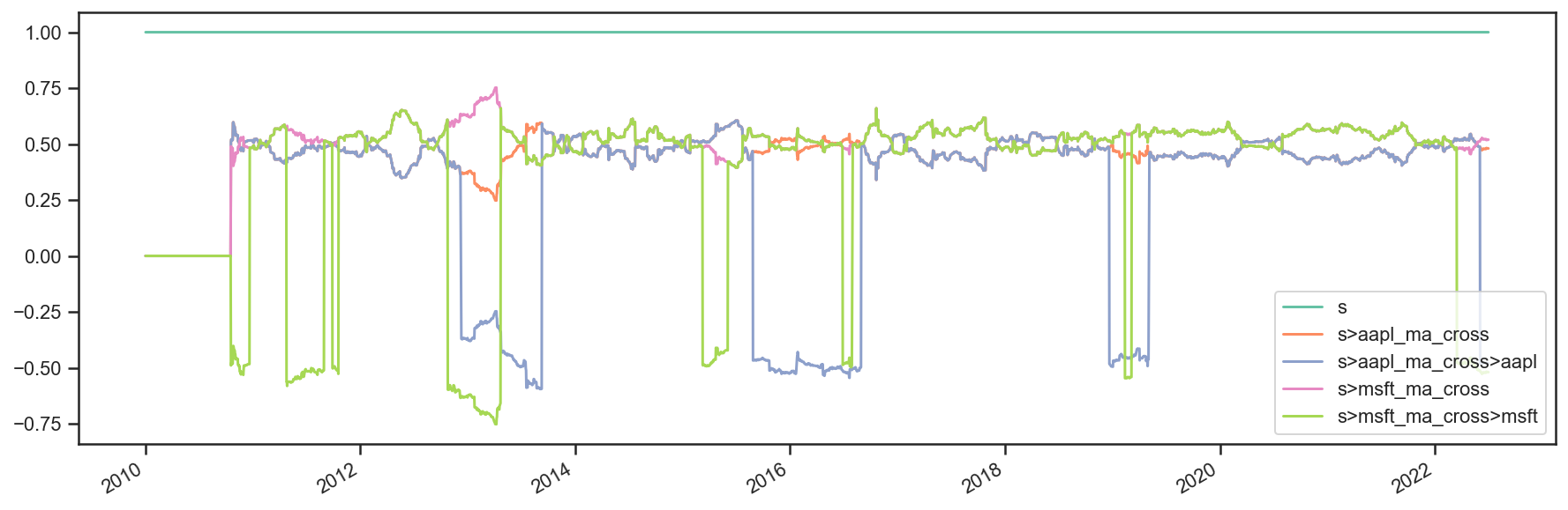
So there you have it. Simpler, and more complete.
Buy and Hold Strategy
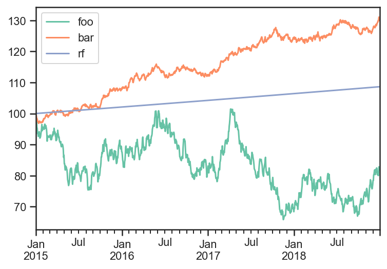
import numpy as np
import pandas as pd
import matplotlib.pyplot as plt

import ffn
import bt

%matplotlib inline
Create Fake Index Data
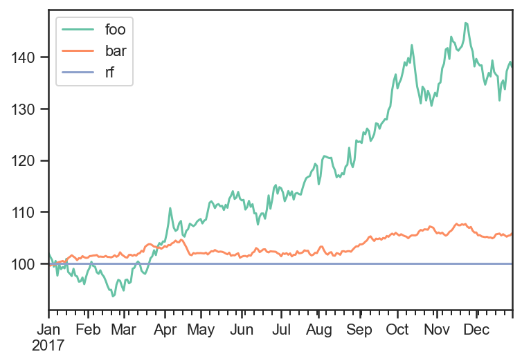
names = ['foo','bar','rf']
dates = pd.date_range(start='2017-01-01',end='2017-12-31', freq=pd.tseries.offsets.BDay())
n = len(dates)
rdf = pd.DataFrame(
    np.zeros((n, len(names))),
    index = dates,
    columns = names
)

np.random.seed(1)
rdf['foo'] = np.random.normal(loc = 0.1/n,scale=0.2/np.sqrt(n),size=n)
rdf['bar'] = np.random.normal(loc = 0.04/n,scale=0.05/np.sqrt(n),size=n)
rdf['rf'] = 0.

pdf = 100*np.cumprod(1+rdf)
pdf.plot();
Build Strategy
# algo to fire on the beginning of every month and to run on the first date
runMonthlyAlgo = bt.algos.RunMonthly(
    run_on_first_date=True
)

# algo to set the weights
#  it will only run when runMonthlyAlgo returns true
#  which only happens on the first of every month
weights = pd.Series([0.6,0.4,0.],index = rdf.columns)
weighSpecifiedAlgo = bt.algos.WeighSpecified(**weights)

# algo to rebalance the current weights to weights set by weighSpecified
#  will only run when weighSpecifiedAlgo returns true
#  which happens every time it runs
rebalAlgo = bt.algos.Rebalance()

# a strategy that rebalances monthly to specified weights
strat = bt.Strategy('static',
    [
        runMonthlyAlgo,
        weighSpecifiedAlgo,
        rebalAlgo
    ]
)
Run Backtest
Note: The logic of the strategy is seperate from the data used in the backtest.
# set integer_positions=False when positions are not required to be integers(round numbers)
backtest = bt.Backtest(
    strat,
    pdf,
    integer_positions=False
)

res = bt.run(backtest)
res.stats
| static | |
|---|---|
| start | 2017-01-01 00:00:00 |
| end | 2017-12-29 00:00:00 |
| rf | 0.0 |
| total_return | 0.229372 |
| cagr | 0.231653 |
| max_drawdown | -0.069257 |
| calmar | 3.344851 |
| mtd | -0.000906 |
| three_month | 0.005975 |
| six_month | 0.142562 |
| ytd | 0.229372 |
| one_year | NaN |
| three_year | NaN |
| five_year | NaN |
| ten_year | NaN |
| incep | 0.231653 |
| daily_sharpe | 1.804549 |
| daily_sortino | 3.306154 |
| daily_mean | 0.206762 |
| daily_vol | 0.114578 |
| daily_skew | 0.012208 |
| daily_kurt | -0.04456 |
| best_day | 0.020402 |
| worst_day | -0.0201 |
| monthly_sharpe | 2.806444 |
| monthly_sortino | 15.352486 |
| monthly_mean | 0.257101 |
| monthly_vol | 0.091611 |
| monthly_skew | 0.753881 |
| monthly_kurt | 0.456278 |
| best_month | 0.073657 |
| worst_month | -0.014592 |
| yearly_sharpe | NaN |
| yearly_sortino | NaN |
| yearly_mean | NaN |
| yearly_vol | NaN |
| yearly_skew | NaN |
| yearly_kurt | NaN |
| best_year | NaN |
| worst_year | NaN |
| avg_drawdown | -0.016052 |
| avg_drawdown_days | 12.695652 |
| avg_up_month | 0.03246 |
| avg_down_month | -0.008001 |
| win_year_perc | NaN |
| twelve_month_win_perc | NaN |
res.prices.head()
| static | |
|---|---|
| 2017-01-01 | 100.000000 |
| 2017-01-02 | 100.000000 |
| 2017-01-03 | 99.384719 |
| 2017-01-04 | 99.121677 |
| 2017-01-05 | 98.316364 |
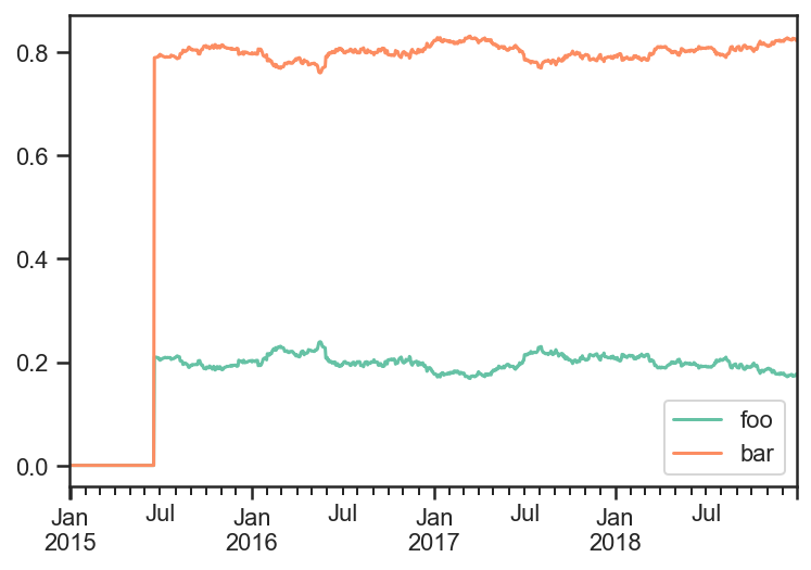
res.plot_security_weights()
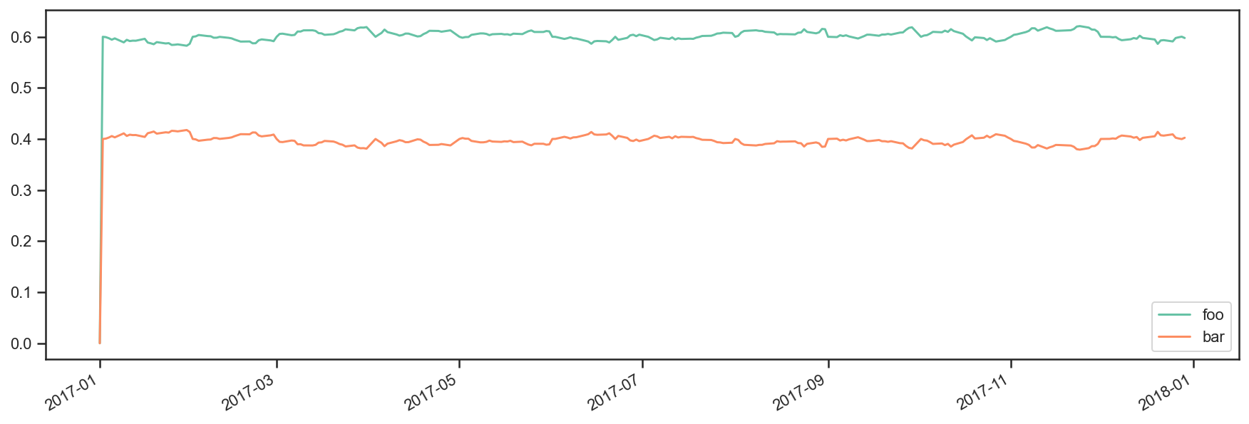
Strategy value over time
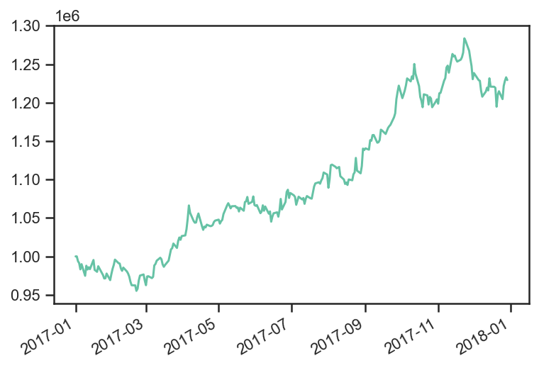
performanceStats = res['static']
#performance stats is an ffn object
res.backtest_list[0].strategy.values.plot();
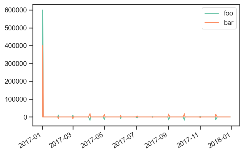
Strategy Outlays
Outlays are the total dollar amount spent(gained) by a purchase(sale) of securities.
res.backtest_list[0].strategy.outlays.plot();
You can get the change in number of shares purchased a
security_names = res.backtest_list[0].strategy.outlays.columns


res.backtest_list[0].strategy.outlays/pdf.loc[:,security_names]
res.backtest_list[0].positions.diff(1)
res.backtest_list[0].positions
| foo | bar | |
|---|---|---|
| 2017-01-01 | 0.000000 | 0.000000 |
| 2017-01-02 | 5879.285683 | 3998.068018 |
| 2017-01-03 | 5879.285683 | 3998.068018 |
| 2017-01-04 | 5879.285683 | 3998.068018 |
| 2017-01-05 | 5879.285683 | 3998.068018 |
| ... | ... | ... |
| 2017-12-25 | 5324.589093 | 4673.239436 |
| 2017-12-26 | 5324.589093 | 4673.239436 |
| 2017-12-27 | 5324.589093 | 4673.239436 |
| 2017-12-28 | 5324.589093 | 4673.239436 |
| 2017-12-29 | 5324.589093 | 4673.239436 |
261 rows × 2 columns
Trend Example 1
import matplotlib.pyplot as plt
import numpy as np
import pandas as pd

import ffn
import bt

%matplotlib inline
Create fake data
rf = 0.04
np.random.seed(1)
mus = np.random.normal(loc=0.05,scale=0.02,size=5) + rf
sigmas = (mus - rf)/0.3 + np.random.normal(loc=0.,scale=0.01,size=5)
num_years = 10
num_months_per_year = 12
num_days_per_month = 21
num_days_per_year = num_months_per_year*num_days_per_month
rdf = pd.DataFrame(
index = pd.date_range(
start="2008-01-02",
periods=num_years*num_months_per_year*num_days_per_month,
freq="B"
),
columns=['foo','bar','baz','fake1','fake2']
)
for i,mu in enumerate(mus):
sigma = sigmas[i]
rdf.iloc[:,i] = np.random.normal(
loc=mu/num_days_per_year,
scale=sigma/np.sqrt(num_days_per_year),
size=rdf.shape[0]
)
pdf = np.cumprod(1+rdf)*100
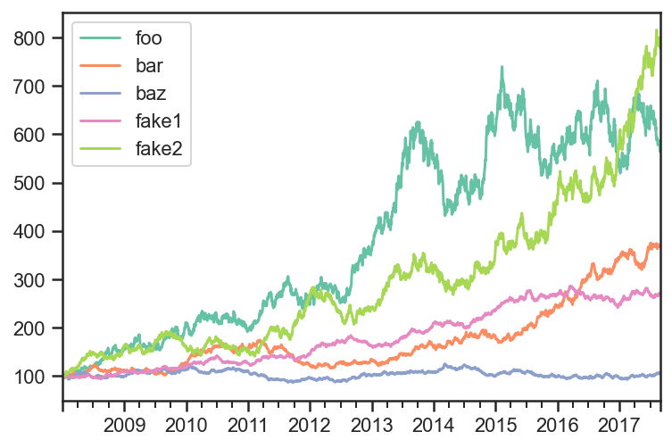
pdf.plot();

Create Trend signal over the last 12 months
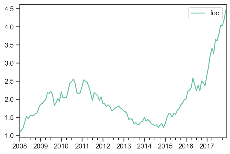
sma  = pdf.rolling(window=num_days_per_month*12,center=False).median().shift(1)
plt.plot(pdf.index,pdf['foo'])
plt.plot(sma.index,sma['foo'])
plt.show()
#sma with 1 day lag
sma.tail()
| foo | bar | baz | fake1 | fake2 | |
|---|---|---|---|---|---|
| 2017-08-23 | 623.241267 | 340.774506 | 99.764885 | 263.491447 | 619.963986 |
| 2017-08-24 | 623.167989 | 341.096742 | 99.764885 | 263.502145 | 620.979948 |
| 2017-08-25 | 622.749149 | 341.316672 | 99.764885 | 263.502145 | 622.421401 |
| 2017-08-28 | 622.353039 | 341.494307 | 99.807732 | 263.517071 | 622.962579 |
| 2017-08-29 | 622.153294 | 341.662442 | 99.807732 | 263.517071 | 622.992416 |
#sma with 0 day lag
pdf.rolling(window=num_days_per_month*12,center=False).median().tail()
| foo | bar | baz | fake1 | fake2 | |
|---|---|---|---|---|---|
| 2017-08-23 | 623.167989 | 341.096742 | 99.764885 | 263.502145 | 620.979948 |
| 2017-08-24 | 622.749149 | 341.316672 | 99.764885 | 263.502145 | 622.421401 |
| 2017-08-25 | 622.353039 | 341.494307 | 99.807732 | 263.517071 | 622.962579 |
| 2017-08-28 | 622.153294 | 341.662442 | 99.807732 | 263.517071 | 622.992416 |
| 2017-08-29 | 621.907867 | 341.948212 | 99.807732 | 263.634283 | 624.310473 |
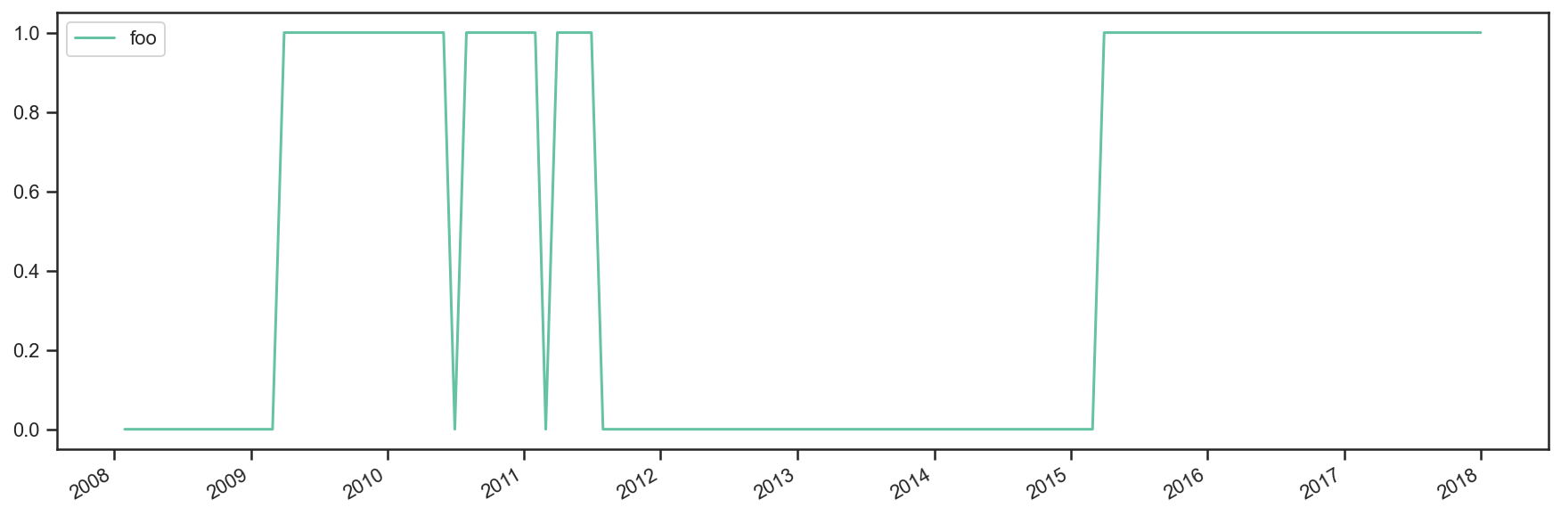
# target weights
trend = sma.copy()
trend[pdf > sma] = True
trend[pdf <= sma] = False
trend[sma.isnull()] = False
trend.tail()
| foo | bar | baz | fake1 | fake2 | |
|---|---|---|---|---|---|
| 2017-08-23 | False | True | True | True | True |
| 2017-08-24 | False | True | True | True | True |
| 2017-08-25 | False | True | True | True | True |
| 2017-08-28 | False | True | True | True | True |
| 2017-08-29 | False | True | True | True | True |
Compare EW and 1/vol
Both strategies rebalance daily using trend with 1 day lag and weights limited to 40%.
tsmom_invvol_strat = bt.Strategy(
    'tsmom_invvol',
    [
        bt.algos.RunDaily(),
        bt.algos.SelectWhere(trend),
        bt.algos.WeighInvVol(),
        bt.algos.LimitWeights(limit=0.4),
        bt.algos.Rebalance()
    ]
)

tsmom_ew_strat = bt.Strategy(
    'tsmom_ew',
    [
        bt.algos.RunDaily(),
        bt.algos.SelectWhere(trend),
        bt.algos.WeighEqually(),
        bt.algos.LimitWeights(limit=0.4),
        bt.algos.Rebalance()
    ]
)
# create and run
tsmom_invvol_bt = bt.Backtest(
    tsmom_invvol_strat,
    pdf,
    initial_capital=50000000.0,
    commissions=lambda q, p: max(100, abs(q) * 0.0021),
    integer_positions=False,
    progress_bar=True
)
tsmom_invvol_res = bt.run(tsmom_invvol_bt)

tsmom_ew_bt = bt.Backtest(
    tsmom_ew_strat,
    pdf,

    initial_capital=50000000.0,
    commissions=lambda q, p: max(100, abs(q) * 0.0021),
    integer_positions=False,
    progress_bar=True
)
tsmom_ew_res = bt.run(tsmom_ew_bt)
 tsmom_invvol
 0% [############################# ] 100% | ETA: 00:00:00tsmom_ew
 0% [############################# ] 100% | ETA: 00:00:00
ax = plt.subplot()
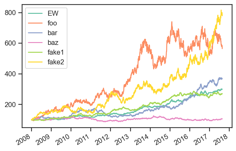
ax.plot(tsmom_ew_res.prices.index,tsmom_ew_res.prices,label='EW')
pdf.plot(ax=ax)
ax.legend()
plt.legend()
plt.show()
tsmom_ew_res.stats
| tsmom_ew | |
|---|---|
| start | 2008-01-01 00:00:00 |
| end | 2017-08-29 00:00:00 |
| rf | 0.0 |
| total_return | 1.982933 |
| cagr | 0.119797 |
| max_drawdown | -0.103421 |
| calmar | 1.158343 |
| mtd | 0.017544 |
| three_month | 0.040722 |
| six_month | 0.079362 |
| ytd | 0.08107 |
| one_year | 0.100432 |
| three_year | 0.159895 |
| five_year | 0.172284 |
| ten_year | 0.119797 |
| incep | 0.119797 |
| daily_sharpe | 1.356727 |
| daily_sortino | 2.332895 |
| daily_mean | 0.112765 |
| daily_vol | 0.083116 |
| daily_skew | 0.029851 |
| daily_kurt | 0.96973 |
| best_day | 0.02107 |
| worst_day | -0.021109 |
| monthly_sharpe | 1.373241 |
| monthly_sortino | 2.966223 |
| monthly_mean | 0.118231 |
| monthly_vol | 0.086096 |
| monthly_skew | -0.059867 |
| monthly_kurt | 0.571064 |
| best_month | 0.070108 |
| worst_month | -0.064743 |
| yearly_sharpe | 1.741129 |
| yearly_sortino | inf |
| yearly_mean | 0.129033 |
| yearly_vol | 0.074109 |
| yearly_skew | 0.990397 |
| yearly_kurt | 1.973883 |
| best_year | 0.285249 |
| worst_year | 0.024152 |
| avg_drawdown | -0.015516 |
| avg_drawdown_days | 25.223214 |
| avg_up_month | 0.024988 |
| avg_down_month | -0.012046 |
| win_year_perc | 1.0 |
| twelve_month_win_perc | 0.971429 |
Trend Example 2
import numpy as np
import pandas as pd

import bt
import matplotlib.pyplot as plt

%matplotlib inline
np.random.seed(0)
returns =  np.random.normal(0.08/12,0.2/np.sqrt(12),12*10)
pdf = pd.DataFrame(
    np.cumprod(1+returns),
    index = pd.date_range(start="2008-01-01",periods=12*10,freq="m"),
    columns=['foo']
)

pdf.plot();
runMonthlyAlgo = bt.algos.RunMonthly()
rebalAlgo = bt.algos.Rebalance()

class Signal(bt.Algo):

    """

    Mostly copied from StatTotalReturn

    Sets temp['Signal'] with total returns over a given period.

    Sets the 'Signal' based on the total return of each
    over a given lookback period.

    Args:
        * lookback (DateOffset): lookback period.
        * lag (DateOffset): Lag interval. Total return is calculated in
            the inteval [now - lookback - lag, now - lag]

    Sets:
        * stat

    Requires:
        * selected

    """

    def __init__(self, lookback=pd.DateOffset(months=3),
                 lag=pd.DateOffset(days=0)):
        super(Signal, self).__init__()
        self.lookback = lookback
        self.lag = lag

    def __call__(self, target):
        selected = 'foo'
        t0 = target.now - self.lag

        if target.universe[selected].index[0] > t0:
            return False
        prc = target.universe[selected].loc[t0 - self.lookback:t0]


        trend = prc.iloc[-1]/prc.iloc[0] - 1
        signal = trend > 0.

        if signal:
            target.temp['Signal'] = 1.
        else:
            target.temp['Signal'] = 0.

        return True

signalAlgo = Signal(pd.DateOffset(months=12),pd.DateOffset(months=1))

class WeighFromSignal(bt.Algo):

    """
    Sets temp['weights'] from the signal.
    Sets:
        * weights

    Requires:
        * selected

    """

    def __init__(self):
        super(WeighFromSignal, self).__init__()

    def __call__(self, target):
        selected = 'foo'
        if target.temp['Signal'] is None:
            raise(Exception('No Signal!'))

        target.temp['weights'] = {selected : target.temp['Signal']}
        return True

weighFromSignalAlgo = WeighFromSignal()
s = bt.Strategy(
    'example1',
    [
        runMonthlyAlgo,
        signalAlgo,
        weighFromSignalAlgo,
        rebalAlgo
    ]
)

t = bt.Backtest(s, pdf, integer_positions=False, progress_bar=True)
res = bt.run(t)
 example1
 0% [############################# ] 100% | ETA: 00:00:00
res.plot_security_weights();
t.positions
| foo | |
|---|---|
| 2008-01-30 | 0.000000 |
| 2008-01-31 | 0.000000 |
| 2008-02-29 | 0.000000 |
| 2008-03-31 | 0.000000 |
| 2008-04-30 | 0.000000 |
| ... | ... |
| 2017-08-31 | 631321.251898 |
| 2017-09-30 | 631321.251898 |
| 2017-10-31 | 631321.251898 |
| 2017-11-30 | 631321.251898 |
| 2017-12-31 | 631321.251898 |
121 rows × 1 columns
res.prices.tail()
| example1 | |
|---|---|
| 2017-08-31 | 240.302579 |
| 2017-09-30 | 255.046653 |
| 2017-10-31 | 254.464421 |
| 2017-11-30 | 265.182603 |
| 2017-12-31 | 281.069771 |
res.stats
| example1 | |
|---|---|
| start | 2008-01-30 00:00:00 |
| end | 2017-12-31 00:00:00 |
| rf | 0.0 |
| total_return | 1.810698 |
| cagr | 0.109805 |
| max_drawdown | -0.267046 |
| calmar | 0.411186 |
| mtd | 0.05991 |
| three_month | 0.102033 |
| six_month | 0.22079 |
| ytd | 0.879847 |
| one_year | 0.879847 |
| three_year | 0.406395 |
| five_year | 0.227148 |
| ten_year | 0.109805 |
| incep | 0.109805 |
| daily_sharpe | 3.299555 |
| daily_sortino | 6.352869 |
| daily_mean | 2.448589 |
| daily_vol | 0.742097 |
| daily_skew | 0.307861 |
| daily_kurt | 1.414455 |
| best_day | 0.137711 |
| worst_day | -0.14073 |
| monthly_sharpe | 0.723148 |
| monthly_sortino | 1.392893 |
| monthly_mean | 0.117579 |
| monthly_vol | 0.162594 |
| monthly_skew | 0.301545 |
| monthly_kurt | 1.379006 |
| best_month | 0.137711 |
| worst_month | -0.14073 |
| yearly_sharpe | 0.503939 |
| yearly_sortino | 5.019272 |
| yearly_mean | 0.14814 |
| yearly_vol | 0.293964 |
| yearly_skew | 2.317496 |
| yearly_kurt | 5.894955 |
| best_year | 0.879847 |
| worst_year | -0.088543 |
| avg_drawdown | -0.091255 |
| avg_drawdown_days | 369.714286 |
| avg_up_month | 0.064341 |
| avg_down_month | -0.012928 |
| win_year_perc | 0.555556 |
| twelve_month_win_perc | 0.46789 |
Strategy Combination
This notebook creates a parent strategy(combined) with 2 child strategies(Equal Weight, Inv Vol).
Alternatively, it creates the 2 child strategies, runs the backtest, combines the results, and creates a parent strategy using both of the backtests.
import numpy as np
import pandas as pd
import matplotlib.pyplot as plt

import ffn
import bt

%matplotlib inline
Create fake data
rf = 0.04
np.random.seed(1)
mus = np.random.normal(loc=0.05,scale=0.02,size=5) + rf
sigmas = (mus - rf)/0.3 + np.random.normal(loc=0.,scale=0.01,size=5)
num_years = 10
num_months_per_year = 12
num_days_per_month = 21
num_days_per_year = num_months_per_year*num_days_per_month
rdf = pd.DataFrame(
index = pd.date_range(
start="2008-01-02",
periods=num_years*num_months_per_year*num_days_per_month,
freq="B"
),
columns=['foo','bar','baz','fake1','fake2']
)
for i,mu in enumerate(mus):
sigma = sigmas[i]
rdf.iloc[:,i] = np.random.normal(
loc=mu/num_days_per_year,
scale=sigma/np.sqrt(num_days_per_year),
size=rdf.shape[0]
)
pdf = np.cumprod(1+rdf)*100
pdf.iloc[0,:] = 100
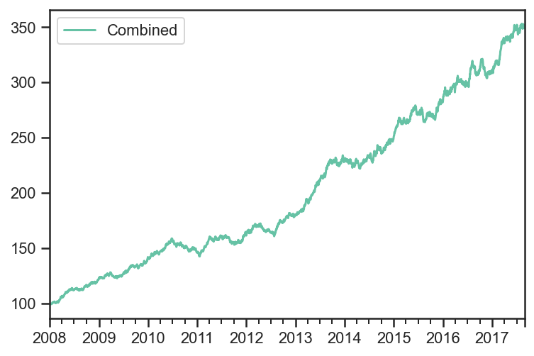
pdf.plot();
strategy_names = np.array(
    [
        'Equal Weight',
        'Inv Vol'
    ]
)

runMonthlyAlgo = bt.algos.RunMonthly(
    run_on_first_date=True,
    run_on_end_of_period=True
)
selectAllAlgo = bt.algos.SelectAll()
rebalanceAlgo = bt.algos.Rebalance()

strats = []
tests = []

for i,s in enumerate(strategy_names):
    if s == "Equal Weight":
        wAlgo = bt.algos.WeighEqually()
    elif s == "Inv Vol":
        wAlgo = bt.algos.WeighInvVol()

    strat = bt.Strategy(
        str(s),
        [
            runMonthlyAlgo,
            selectAllAlgo,
            wAlgo,
            rebalanceAlgo
        ]
    )
    strats.append(strat)

    t = bt.Backtest(
        strat,
        pdf,
        integer_positions = False,
        progress_bar=False
    )
    tests.append(t)
combined_strategy = bt.Strategy(
    'Combined',
    algos = [
        runMonthlyAlgo,
        selectAllAlgo,
        bt.algos.WeighEqually(),
        rebalanceAlgo
    ],
    children = [x.strategy for x in tests]
)

combined_test = bt.Backtest(
    combined_strategy,
    pdf,
    integer_positions = False,
    progress_bar = False
)

res = bt.run(combined_test)
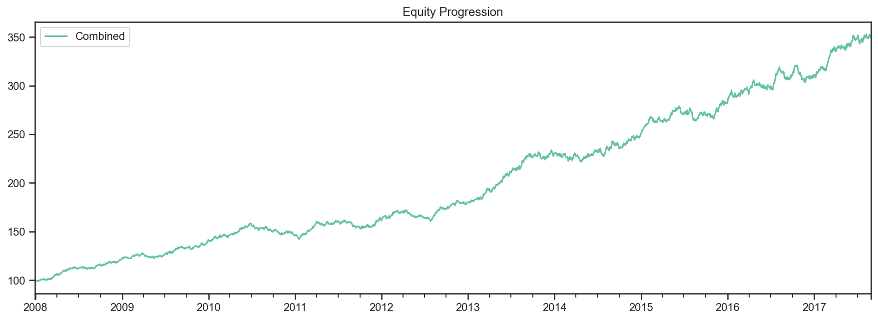
res.prices.plot();
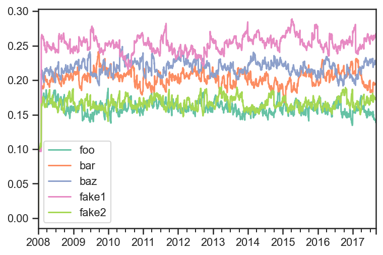
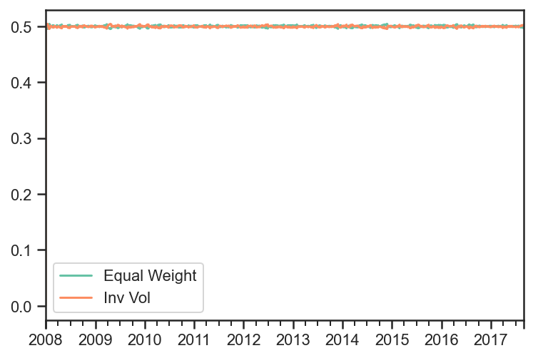
res.get_security_weights().plot();
In order to get the weights of each strategy, you can run each strategy, get the prices for each strategy, combine them into one price dataframe, run the combined strategy on the new data set.
strategy_names = np.array(
    [
        'Equal Weight',
        'Inv Vol'
    ]
)

runMonthlyAlgo = bt.algos.RunMonthly(
    run_on_first_date=True,
    run_on_end_of_period=True
)
selectAllAlgo = bt.algos.SelectAll()
rebalanceAlgo = bt.algos.Rebalance()

strats = []
tests = []
results = []

for i,s in enumerate(strategy_names):
    if s == "Equal Weight":
        wAlgo = bt.algos.WeighEqually()
    elif s == "Inv Vol":
        wAlgo = bt.algos.WeighInvVol()

    strat = bt.Strategy(
        s,
        [
            runMonthlyAlgo,
            selectAllAlgo,
            wAlgo,
            rebalanceAlgo
        ]
    )
    strats.append(strat)

    t = bt.Backtest(
        strat,
        pdf,
        integer_positions = False,
        progress_bar=False
    )
    tests.append(t)

    res = bt.run(t)
    results.append(res)
fig, ax = plt.subplots(nrows=1,ncols=1)
for i,r in enumerate(results):
    r.plot(ax=ax)
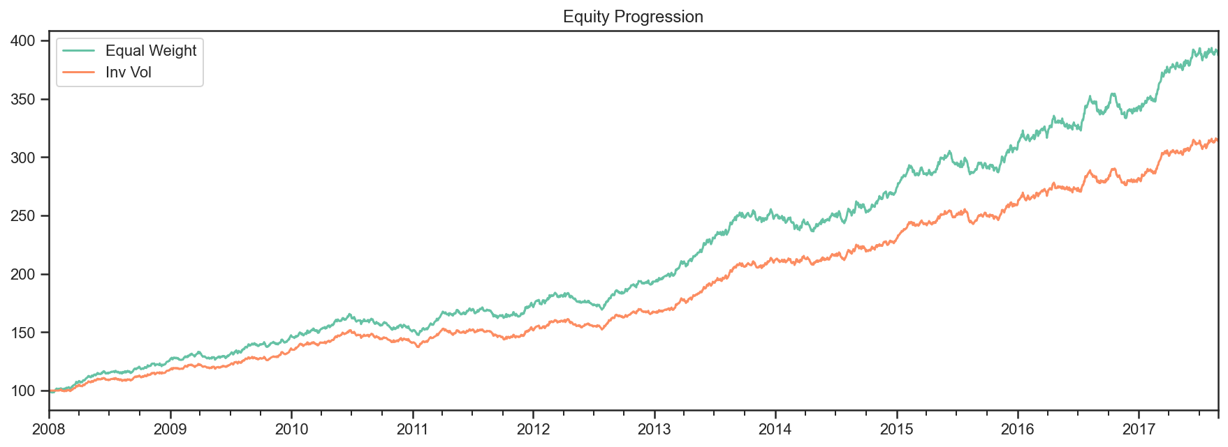
merged_prices_df = bt.merge(results[0].prices,results[1].prices)

combined_strategy = bt.Strategy(
    'Combined',
    algos = [
        runMonthlyAlgo,
        selectAllAlgo,
        bt.algos.WeighEqually(),
        rebalanceAlgo
    ]
)

combined_test = bt.Backtest(
    combined_strategy,
    merged_prices_df,
    integer_positions = False,
    progress_bar = False
)

res = bt.run(combined_test)
res.plot();
res.get_security_weights().plot();
Equally Weighted Risk Contributions Portfolio
import numpy as np
import pandas as pd
import matplotlib.pyplot as plt

import ffn
import bt

%matplotlib inline
Create Fake Index Data
mean = np.array([0.05/252 + 0.02/252, 0.03/252 + 0.02/252])
volatility = np.array([0.2/np.sqrt(252), 0.05/np.sqrt(252)])
variance = np.power(volatility,2)
correlation = np.array(
    [
        [1, 0.25],
        [0.25,1]
    ]
)
covariance = np.zeros((2,2))
for i in range(len(variance)):
    for j in range(len(variance)):
        covariance[i,j] = correlation[i,j]*volatility[i]*volatility[j]

covariance
 array([[1.58730159e-04, 9.92063492e-06],
        [9.92063492e-06, 9.92063492e-06]])
names = ['foo','bar','rf']
dates = pd.date_range(start='2015-01-01',end='2018-12-31', freq=pd.tseries.offsets.BDay())
n = len(dates)
rdf = pd.DataFrame(
    np.zeros((n, len(names))),
    index = dates,
    columns = names
)

np.random.seed(1)
rdf.loc[:,['foo','bar']] = np.random.multivariate_normal(mean,covariance,size=n)
rdf['rf'] = 0.02/252

pdf = 100*np.cumprod(1+rdf)
pdf.plot();
Build and run ERC Strategy
You can read more about ERC here. http://thierry-roncalli.com/download/erc.pdf
runAfterDaysAlgo = bt.algos.RunAfterDays(
    20*6 + 1
)

selectTheseAlgo = bt.algos.SelectThese(['foo','bar'])

# algo to set the weights so each asset contributes the same amount of risk
#  with data over the last 6 months excluding yesterday
weighERCAlgo = bt.algos.WeighERC(
    lookback=pd.DateOffset(days=20*6),
    covar_method='standard',
    risk_parity_method='slsqp',
    maximum_iterations=1000,
    tolerance=1e-9,
    lag=pd.DateOffset(days=1)
)

rebalAlgo = bt.algos.Rebalance()

strat = bt.Strategy(
    'ERC',
    [
        runAfterDaysAlgo,
        selectTheseAlgo,
        weighERCAlgo,
        rebalAlgo
    ]
)

backtest = bt.Backtest(
    strat,
    pdf,
    integer_positions=False
)

res_target = bt.run(backtest)
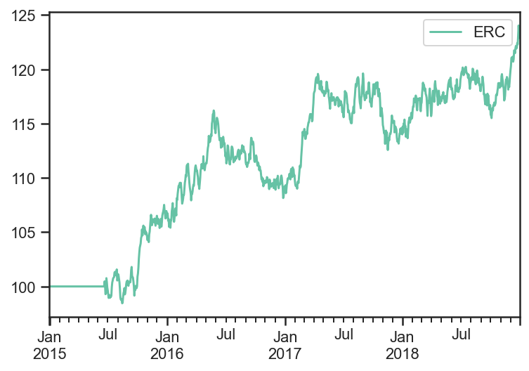
res_target.get_security_weights().plot();
res_target.prices.plot();
weights_target = res_target.get_security_weights().copy()
rolling_cov_target = pdf.loc[:,weights_target.columns].pct_change().rolling(window=252).cov()*252


trc_target = pd.DataFrame(
    np.nan,
    index = weights_target.index,
    columns = weights_target.columns
)

for dt in pdf.index:
    trc_target.loc[dt,:] = weights_target.loc[dt,:].values*(rolling_cov_target.loc[dt,:].values@weights_target.loc[dt,:].values)/np.sqrt(weights_target.loc[dt,:].values@rolling_cov_target.loc[dt,:].values@weights_target.loc[dt,:].values)


fig, ax = plt.subplots(nrows=1,ncols=1)
trc_target.plot(ax=ax)
ax.set_title('Total Risk Contribution')
ax.plot();
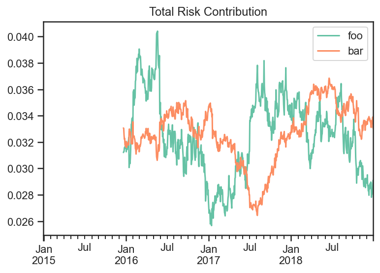
You can see the Total Risk Contribution is roughly equal from both assets.
Predicted Tracking Error Rebalance Portfolio
import numpy as np
import pandas as pd
import matplotlib.pyplot as plt

import ffn
import bt

%matplotlib inline
Create Fake Index Data
names = ['foo','bar','rf']
dates = pd.date_range(start='2015-01-01',end='2018-12-31', freq=pd.tseries.offsets.BDay())
n = len(dates)
rdf = pd.DataFrame(
    np.zeros((n, len(names))),
    index = dates,
    columns = names
)

np.random.seed(1)
rdf['foo'] = np.random.normal(loc = 0.1/252,scale=0.2/np.sqrt(252),size=n)
rdf['bar'] = np.random.normal(loc = 0.04/252,scale=0.05/np.sqrt(252),size=n)
rdf['rf'] = 0.

pdf = 100*np.cumprod(1+rdf)
pdf.plot();
Build and run Target Strategy
I will first run a strategy that rebalances everyday.
Then I will use those weights as target to rebalance to whenever the PTE is too high.
selectTheseAlgo = bt.algos.SelectThese(['foo','bar'])

# algo to set the weights to 1/vol contributions from each asset
#  with data over the last 3 months excluding yesterday
weighInvVolAlgo = bt.algos.WeighInvVol(
    lookback=pd.DateOffset(months=3),
    lag=pd.DateOffset(days=1)
)

# algo to rebalance the current weights to weights set in target.temp
rebalAlgo = bt.algos.Rebalance()

# a strategy that rebalances daily to 1/vol weights
strat = bt.Strategy(
    'Target',
    [
        selectTheseAlgo,
        weighInvVolAlgo,
        rebalAlgo
    ]
)

# set integer_positions=False when positions are not required to be integers(round numbers)
backtest = bt.Backtest(
    strat,
    pdf,
    integer_positions=False
)

res_target = bt.run(backtest)
res_target.get_security_weights().plot();
Now use the PTE rebalance algo to trigger a rebalance whenever predicted tracking error is greater than 1%.
# algo to fire whenever predicted tracking error is greater than 1%
wdf = res_target.get_security_weights()

PTE_rebalance_Algo = bt.algos.PTE_Rebalance(
    0.01,
    wdf,
    lookback=pd.DateOffset(months=3),
    lag=pd.DateOffset(days=1),
    covar_method='standard',
    annualization_factor=252
)

selectTheseAlgo = bt.algos.SelectThese(['foo','bar'])

# algo to set the weights to 1/vol contributions from each asset
#  with data over the last 12 months excluding yesterday
weighTargetAlgo = bt.algos.WeighTarget(
    wdf
)

rebalAlgo = bt.algos.Rebalance()

# a strategy that rebalances monthly to specified weights
strat = bt.Strategy(
    'PTE',
    [
        PTE_rebalance_Algo,
        selectTheseAlgo,
        weighTargetAlgo,
        rebalAlgo
    ]
)

# set integer_positions=False when positions are not required to be integers(round numbers)
backtest = bt.Backtest(
    strat,
    pdf,
    integer_positions=False
)

res_PTE = bt.run(backtest)
fig, ax = plt.subplots(nrows=1,ncols=1)
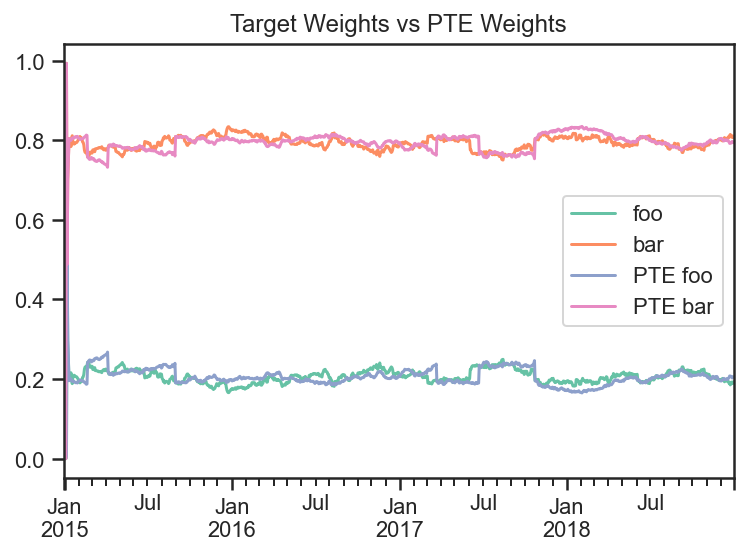
res_target.get_security_weights().plot(ax=ax)
realized_weights_df = res_PTE.get_security_weights()
realized_weights_df['PTE foo'] = realized_weights_df['foo']
realized_weights_df['PTE bar'] = realized_weights_df['bar']
realized_weights_df = realized_weights_df.loc[:,['PTE foo', 'PTE bar']]
realized_weights_df.plot(ax=ax)
ax.set_title('Target Weights vs PTE Weights')
ax.plot();
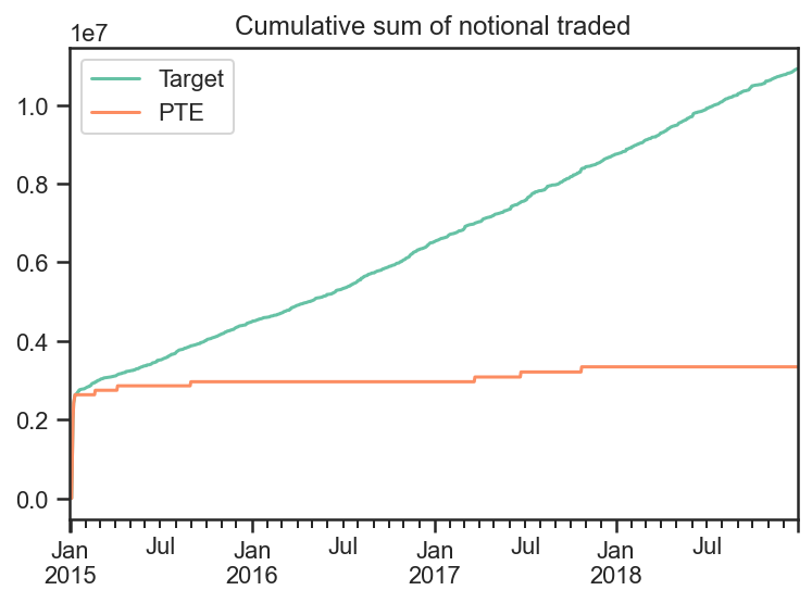
trans_df = pd.DataFrame(
    index=res_target.prices.index,
    columns=['Target','PTE']
)

transactions = res_target.get_transactions()
transactions = (transactions['quantity'] * transactions['price']).reset_index()

bar_mask = transactions.loc[:,'Security'] == 'bar'
foo_mask = transactions.loc[:,'Security'] == 'foo'

trans_df.loc[trans_df.index[4:],'Target'] = np.abs(transactions[bar_mask].iloc[:,2].values) + np.abs(transactions[foo_mask].iloc[:,2].values)
transactions = res_PTE.get_transactions()
transactions = (transactions['quantity'] * transactions['price']).reset_index()

bar_mask = transactions.loc[:,'Security'] == 'bar'
foo_mask = transactions.loc[:,'Security'] == 'foo'

trans_df.loc[transactions[bar_mask].iloc[:,0],'PTE'] =  np.abs(transactions[bar_mask].iloc[:,2].values)
trans_df.loc[transactions[foo_mask].iloc[:,0],'PTE'] +=  np.abs(transactions[foo_mask].iloc[:,2].values)
trans_df = trans_df.fillna(0)
fig, ax = plt.subplots(nrows=1,ncols=1)
trans_df.cumsum().plot(ax=ax)
ax.set_title('Cumulative sum of notional traded')
ax.plot();
If we plot the total risk contribution of each asset class and divide by the total volatility, then we can see that both strategy’s contribute roughly similar amounts of volatility from both of the securities.
weights_target = res_target.get_security_weights()
rolling_cov_target = pdf.loc[:,weights_target.columns].pct_change().rolling(window=3*20).cov()*252

weights_PTE = res_PTE.get_security_weights().loc[:,weights_target.columns]
rolling_cov_PTE = pdf.loc[:,weights_target.columns].pct_change().rolling(window=3*20).cov()*252


trc_target = pd.DataFrame(
    np.nan,
    index = weights_target.index,
    columns = weights_target.columns
)

trc_PTE = pd.DataFrame(
    np.nan,
    index = weights_PTE.index,
    columns = [x + " PTE" for x in weights_PTE.columns]
)

for dt in pdf.index:
    trc_target.loc[dt,:] = weights_target.loc[dt,:].values*(rolling_cov_target.loc[dt,:].values@weights_target.loc[dt,:].values)/np.sqrt(weights_target.loc[dt,:].values@rolling_cov_target.loc[dt,:].values@weights_target.loc[dt,:].values)
    trc_PTE.loc[dt,:] = weights_PTE.loc[dt,:].values*(rolling_cov_PTE.loc[dt,:].values@weights_PTE.loc[dt,:].values)/np.sqrt(weights_PTE.loc[dt,:].values@rolling_cov_PTE.loc[dt,:].values@weights_PTE.loc[dt,:].values)


fig, ax = plt.subplots(nrows=1,ncols=1)
trc_target.plot(ax=ax)
trc_PTE.plot(ax=ax)
ax.set_title('Total Risk Contribution')
ax.plot();
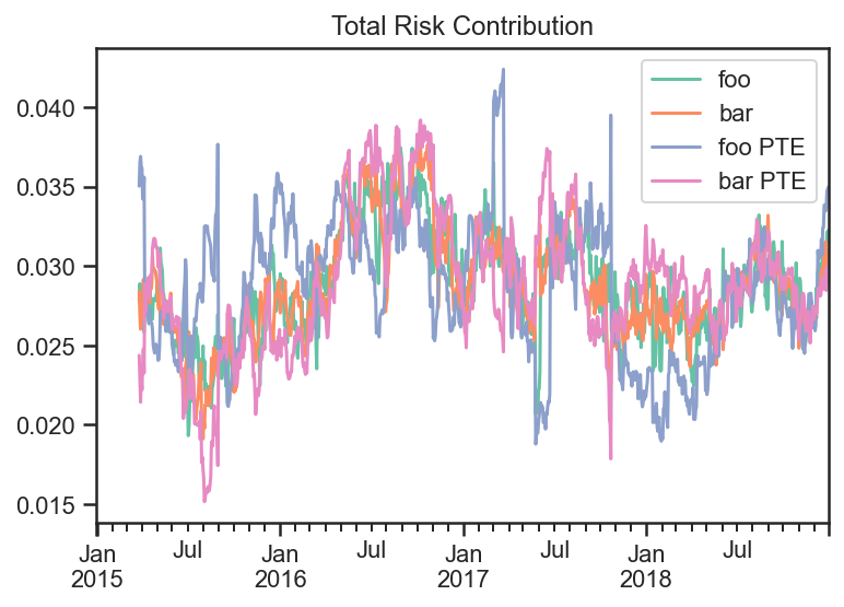
Looking at the Target strategy’s and PTE strategy’s Total Risk they are very similar.
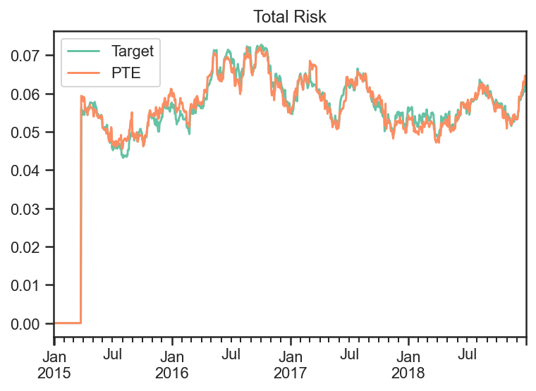
fig, ax = plt.subplots(nrows=1,ncols=1)
trc_target.sum(axis=1).plot(ax=ax,label='Target')
trc_PTE.sum(axis=1).plot(ax=ax,label='PTE')
ax.legend()
ax.set_title('Total Risk')
ax.plot();
transactions = res_PTE.get_transactions()
transactions = (transactions['quantity'] * transactions['price']).reset_index()

bar_mask = transactions.loc[:,'Security'] == 'bar'
dates_of_PTE_transactions = transactions[bar_mask].iloc[:,0]
dates_of_PTE_transactions
 0    2015-01-06
 2    2015-01-07
 4    2015-01-08
 6    2015-01-09
 8    2015-01-12
 10   2015-02-20
 12   2015-04-07
 14   2015-09-01
 16   2017-03-23
 18   2017-06-23
 20   2017-10-24
 Name: Date, dtype: datetime64[ns]
fig, ax = plt.subplots(nrows=1,ncols=1)
np.sum(np.abs(trc_target.values - trc_PTE.values))
    #.abs().sum(axis=1).plot()

ax.set_title('Total Risk')
ax.plot(
    trc_target.index,
    np.sum(np.abs(trc_target.values - trc_PTE.values),axis=1),
    label='PTE'
)

for i,dt in enumerate(dates_of_PTE_transactions):
    if i == 0:
        ax.axvline(x=dt,color='red',label='PTE Transaction')
    else:
        ax.axvline(x=dt,color='red')

ax.legend();
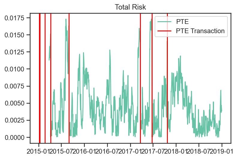
We can see the Predicted Tracking Error of the PTE Strategy with each transaction marked.
Fixed Income Examples
This example notebook illustrates some of the more sophisticated functionality of the package, especially related to fixed income securities and strategies. For fixed income strategies:
capital allocations are not necessary, and initial capital is not used
bankruptcy is disabled (as money can always be borrowed at some rate, potentially represented as another asset)
weights are based off notional_value rather than value. For fixed income securities, notional value is just the position. For non-fixed income securities (i.e. equities), it is the market value of the position.
strategy notional_value is always positive, equal to the sum of the magnitudes of the notional values of all its children
strategy price is computed from additive PNL returns per unit of notional_value, with a reference price of PAR
“rebalancing” the portfolio adjusts notionals rather than capital allocations based on weights
Further to the above characteristics of fixed income strategies, we also demonstrate the usage of the following features which arise in these types of use case:
Coupon paying securities (i.e. bonds)
Handing of security lifecycle such as new issues and maturity
Usage of “On-The-Run” instruments, and rolling of positions into the “new” on-the-run security at pre-defined times
Risk tracking/aggregation and hedging from pre-computed risk per unit notional
The notebook contains the following parts:
Setup
Market data generation
Rolling series of government bonds
Corporate bonds with spreads driven by a common factor
Example 1: Basic Strategies
Weigh all active corporate bond equally
Add hedging of interest rates risk with the on-the-run government bond
Example 2: Nested Strategies
One strategy buys the top N bonds, by yield
Another strategy sells the bottom N bonds, by yield
Parent strategy gives 50% weight to each of the above
Add hedges of remaining interest rates risk with the on-the-run government bond
Setup
import bt
import pandas as pd
from pandas.tseries.frequencies import to_offset
import numpy as np
np.random.seed(1234)
%matplotlib inline
# (Approximate) Price to yield calcs, and pvbp, for later use. Note we use clean price here.
def price_to_yield( p, ttm, coupon ):
    return ( coupon + (100. - p)/ttm ) / ( ( 100. + p)/2. ) * 100
def yield_to_price( y, ttm, coupon ):
    return (coupon + 100/ttm - 0.5 * y) / ( y/200 + 1/ttm)
def pvbp( y, ttm, coupon ):
    return (yield_to_price( y + 0.01, ttm, coupon ) - yield_to_price( y, ttm, coupon ))
# Utility function to set data frame values to nan before the security has been issued or after it has matured
def censor( data, ref_data ):
    for bond in data:
        data.loc[ (data.index > ref_data['mat_date'][bond]) | (data.index < ref_data['issue_date'][bond]), bond] = np.NaN
    return data.ffill(limit=1,axis=0) # Because bonds might mature during a gap in the index (i.e. on the weekend)
# Backtesting timeline setup
start_date = pd.Timestamp('2020-01-01')
end_date = pd.Timestamp('2022-01-01')
timeline = pd.date_range( start_date, end_date, freq='B')
Market Data Generation
# Government Bonds: Create synthetic data for a single series of rolling government bonds

# Reference Data
roll_freq = 'Q'
maturity = 10
coupon = 2.0
roll_dates = pd.date_range( start_date, end_date+to_offset(roll_freq), freq=roll_freq) # Go one period beyond the end date to be safe
issue_dates = roll_dates - roll_dates.freq
mat_dates = issue_dates + pd.offsets.DateOffset(years=maturity)
series_name = 'govt_10Y'
names = pd.Series(mat_dates).apply( lambda x : 'govt_%s' % x.strftime('%Y_%m'))
# Build a time series of OTR
govt_otr = pd.DataFrame( [ [ name for name, roll_date in zip(names, roll_dates) if roll_date >=d ][0] for d in timeline ],
                        index=timeline,
                        columns=[series_name])
# Create a data frame of reference data
govt_data = pd.DataFrame( {'mat_date':mat_dates, 'issue_date': issue_dates, 'roll_date':roll_dates}, index = names)
govt_data['coupon'] = coupon

# Create the "roll map"
govt_roll_map = govt_otr.copy()
govt_roll_map['target'] = govt_otr[series_name].shift(-1)
govt_roll_map = govt_roll_map[ govt_roll_map[series_name] != govt_roll_map['target']]
govt_roll_map['factor'] = 1.
govt_roll_map = govt_roll_map.reset_index().set_index(series_name).rename(columns={'index':'date'}).dropna()

# Market Data and Risk
govt_yield_initial = 2.0
govt_yield_vol = 1.
govt_yield = pd.DataFrame( columns = govt_data.index, index=timeline )
govt_yield_ts = (govt_yield_initial + np.cumsum( np.random.normal( 0., govt_yield_vol/np.sqrt(252), len(timeline)))).reshape(-1,1)
govt_yield.loc[:,:] = govt_yield_ts

govt_mat = pd.DataFrame( columns = govt_data.index, index=timeline, data=pd.NA ).astype('datetime64')
govt_mat.loc[:,:] = govt_data['mat_date'].values.T
govt_ttm = (govt_mat - timeline.values.reshape(-1,1))/pd.Timedelta('1Y')
govt_coupon = pd.DataFrame( columns = govt_data.index, index=timeline )
govt_coupon.loc[:,:] = govt_data['coupon'].values.T
govt_accrued = govt_coupon.multiply( timeline.to_series().diff()/pd.Timedelta('1Y'), axis=0 )
govt_accrued.iloc[0] = 0

govt_price = yield_to_price( govt_yield, govt_ttm, govt_coupon )
govt_price[ govt_ttm <= 0 ] = 100.
govt_price = censor(govt_price, govt_data)
govt_pvbp = pvbp( govt_yield, govt_ttm, govt_coupon)
govt_pvbp[ govt_ttm <= 0 ] = 0.
govt_pvbp = censor(govt_pvbp, govt_data)
 /opt/homebrew/lib/python3.9/site-packages/IPython/core/interactiveshell.py:3397: FutureWarning: Units 'M', 'Y' and 'y' do not represent unambiguous timedelta values and will be removed in a future version
   exec(code_obj, self.user_global_ns, self.user_ns)
# Corporate Bonds: Create synthetic data for a universe of corporate bonds

# Reference Data
n_corp = 50    # Number of corporate bonds to generate
avg_ttm = 10   # Average time to maturity, in years
coupon_mean = 5
coupon_std = 1.5
mat_dates = start_date + np.random.exponential(avg_ttm*365, n_corp).astype(int) * pd.offsets.Day()
issue_dates = np.minimum( mat_dates, end_date ) - np.random.exponential(avg_ttm*365, n_corp).astype(int) * pd.offsets.Day()
names = pd.Series( [ 'corp{:04d}'.format(i) for i in range(n_corp)])
coupons = np.random.normal( coupon_mean, coupon_std, n_corp ).round(3)
corp_data = pd.DataFrame( {'mat_date':mat_dates, 'issue_date': issue_dates, 'coupon':coupons}, index=names)

# Market Data and Risk
# Model: corporate yield = government yield + credit spread
# Model: credit spread changes = beta * common factor changes + idiosyncratic changes
corp_spread_initial = np.random.normal( 2, 1, len(corp_data) )
corp_betas_raw = np.random.normal( 1, 0.5, len(corp_data) )
corp_factor_vol = 0.5
corp_idio_vol = 0.5
corp_factor_ts = np.cumsum( np.random.normal( 0, corp_factor_vol/np.sqrt(252), len(timeline))).reshape(-1,1)
corp_idio_ts = np.cumsum( np.random.normal( 0, corp_idio_vol/np.sqrt(252), len(timeline))).reshape(-1,1)
corp_spread = corp_spread_initial + np.multiply( corp_factor_ts, corp_betas_raw ) + corp_idio_ts
corp_yield = govt_yield_ts + corp_spread
corp_yield = pd.DataFrame(  columns = corp_data.index, index=timeline, data = corp_yield )

corp_mat = pd.DataFrame( columns = corp_data.index, index=timeline, data=start_date )
corp_mat.loc[:,:] = corp_data['mat_date'].values.T
corp_ttm = (corp_mat - timeline.values.reshape(-1,1))/pd.Timedelta('1Y')
corp_coupon = pd.DataFrame( columns = corp_data.index, index=timeline )
corp_coupon.loc[:,:] = corp_data['coupon'].values.T
corp_accrued = corp_coupon.multiply( timeline.to_series().diff()/pd.Timedelta('1Y'), axis=0 )
corp_accrued.iloc[0] = 0

corp_price = yield_to_price( corp_yield, corp_ttm, corp_coupon )
corp_price[ corp_ttm <= 0 ] = 100.
corp_price = censor(corp_price, corp_data)

corp_pvbp = pvbp( corp_yield, corp_ttm, corp_coupon)
corp_pvbp[ corp_ttm <= 0 ] = 0.
corp_pvbp = censor(corp_pvbp, corp_data)

bidoffer_bps = 5.
corp_bidoffer = -bidoffer_bps * corp_pvbp

corp_betas = pd.DataFrame( columns = corp_data.index, index=timeline )
corp_betas.loc[:,:] = corp_betas_raw
corp_betas = censor(corp_betas, corp_data)
 /opt/homebrew/lib/python3.9/site-packages/IPython/core/interactiveshell.py:3397: FutureWarning: Units 'M', 'Y' and 'y' do not represent unambiguous timedelta values and will be removed in a future version
   exec(code_obj, self.user_global_ns, self.user_ns)
Example 1: Basic Strategies
# Set up a strategy and a backtest

# The goal here is to define an equal weighted portfolio of corporate bonds,
# and to hedge the rates risk with the rolling series of government bonds

# Define Algo Stacks as the various building blocks
# Note that the order in which we execute these is extremely important

lifecycle_stack = bt.core.AlgoStack(
    # Close any matured bond positions (including hedges)
    bt.algos.ClosePositionsAfterDates( 'maturity' ),
    # Roll government bond positions into the On The Run
    bt.algos.RollPositionsAfterDates( 'govt_roll_map' ),
)
risk_stack = bt.AlgoStack(
    # Specify how frequently to calculate risk
    bt.algos.Or( [bt.algos.RunWeekly(),
                  bt.algos.RunMonthly()] ),
    # Update the risk given any positions that have been put on so far in the current step
    bt.algos.UpdateRisk( 'pvbp', history=1),
    bt.algos.UpdateRisk( 'beta', history=1),
)
hedging_stack = bt.AlgoStack(
    # Specify how frequently to hedge risk
    bt.algos.RunMonthly(),
    # Select the "alias" for the on-the-run government bond...
    bt.algos.SelectThese( [series_name], include_no_data = True ),
    # ... and then resolve it to the underlying security for the given date
    bt.algos.ResolveOnTheRun( 'govt_otr' ),
    # Hedge out the pvbp risk using the selected government bond
    bt.algos.HedgeRisks( ['pvbp']),
    # Need to update risk again after hedging so that it gets recorded correctly (post-hedges)
    bt.algos.UpdateRisk( 'pvbp', history=True),
)
debug_stack = bt.core.AlgoStack(
    # Specify how frequently to display debug info
    bt.algos.RunMonthly(),
    bt.algos.PrintInfo('Strategy {name} : {now}.\tNotional:  {_notl_value:0.0f},\t Value: {_value:0.0f},\t Price: {_price:0.4f}'),
    bt.algos.PrintRisk('Risk: \tPVBP: {pvbp:0.0f},\t Beta: {beta:0.0f}'),
)
trading_stack =bt.core.AlgoStack(
         # Specify how frequently to rebalance the portfolio
         bt.algos.RunMonthly(),
         # Select instruments for rebalancing. Start with everything
         bt.algos.SelectAll(),
         # Prevent matured/rolled instruments from coming back into the mix
         bt.algos.SelectActive(),
         # Select only corp instruments
         bt.algos.SelectRegex( 'corp' ),
         # Specify how to weigh the securities
         bt.algos.WeighEqually(),
         # Set the target portfolio size
         bt.algos.SetNotional( 'notional_value' ),
         # Rebalance the portfolio
         bt.algos.Rebalance()
)

govt_securities = [ bt.CouponPayingHedgeSecurity( name ) for name in govt_data.index]
corp_securities = [ bt.CouponPayingSecurity( name ) for name in corp_data.index ]
securities = govt_securities + corp_securities
base_strategy = bt.FixedIncomeStrategy('BaseStrategy', [ lifecycle_stack, bt.algos.Or( [trading_stack, risk_stack, debug_stack ] ) ], children = securities)
hedged_strategy = bt.FixedIncomeStrategy('HedgedStrategy', [ lifecycle_stack, bt.algos.Or( [trading_stack, risk_stack, hedging_stack, debug_stack ] ) ], children = securities)

#Collect all the data for the strategies

# Here we use clean prices as the data and accrued as the coupon. Could alternatively use dirty prices and cashflows.
data = pd.concat( [ govt_price, corp_price ], axis=1) / 100.  # Because we need prices per unit notional
additional_data = { 'coupons' : pd.concat([govt_accrued, corp_accrued], axis=1) / 100.,
                   'bidoffer' : corp_bidoffer/100.,
                   'notional_value' : pd.Series( data=1e6, index=data.index ),
                   'maturity' : pd.concat([govt_data, corp_data], axis=0).rename(columns={"mat_date": "date"}),
                   'govt_roll_map' : govt_roll_map,
                   'govt_otr' : govt_otr,
                   'unit_risk' : {'pvbp' : pd.concat( [ govt_pvbp, corp_pvbp] ,axis=1)/100.,
                                  'beta' : corp_betas * corp_pvbp / 100.},
                  }
base_test = bt.Backtest( base_strategy, data, 'BaseBacktest',
                initial_capital = 0,
                additional_data = additional_data )
hedge_test = bt.Backtest( hedged_strategy, data, 'HedgedBacktest',
                initial_capital = 0,
                additional_data = additional_data)
out = bt.run( base_test, hedge_test )
 Strategy BaseStrategy : 2020-01-01 00:00:00.        Notional:  1000000,      Value: -1644,   Price: 99.8356
 Risk:       PVBP: -658,      Beta: -659
 Strategy BaseStrategy : 2020-02-03 00:00:00.        Notional:  1000000,      Value: -6454,   Price: 99.3546
 Risk:       PVBP: -642,      Beta: -643
 Strategy BaseStrategy : 2020-03-02 00:00:00.        Notional:  1000000,      Value: -26488,  Price: 97.3512
 Risk:       PVBP: -611,      Beta: -613
 Strategy BaseStrategy : 2020-04-01 00:00:00.        Notional:  1000000,      Value: -20295,  Price: 97.9705
 Risk:       PVBP: -607,      Beta: -608
 Strategy BaseStrategy : 2020-05-01 00:00:00.        Notional:  1000000,      Value: -43692,  Price: 95.6308
 Risk:       PVBP: -573,      Beta: -574
 Strategy BaseStrategy : 2020-06-01 00:00:00.        Notional:  1000000,      Value: -41095,  Price: 95.8905
 Risk:       PVBP: -566,      Beta: -566
 Strategy BaseStrategy : 2020-07-01 00:00:00.        Notional:  1000000,      Value: -15724,  Price: 98.4985
 Risk:       PVBP: -609,      Beta: -608
 Strategy BaseStrategy : 2020-08-03 00:00:00.        Notional:  1000000,      Value: -22308,  Price: 97.8400
 Risk:       PVBP: -587,      Beta: -594
 Strategy BaseStrategy : 2020-09-01 00:00:00.        Notional:  1000000,      Value: 12832,   Price: 101.4263
 Risk:       PVBP: -644,      Beta: -650
 Strategy BaseStrategy : 2020-10-01 00:00:00.        Notional:  1000000,      Value: 35263,   Price: 103.6965
 Risk:       PVBP: -683,      Beta: -680
 Strategy BaseStrategy : 2020-11-02 00:00:00.        Notional:  1000000,      Value: 3702,    Price: 100.5404
 Risk:       PVBP: -638,      Beta: -646
 Strategy BaseStrategy : 2020-12-01 00:00:00.        Notional:  1000000,      Value: -18534,  Price: 98.3168
 Risk:       PVBP: -606,      Beta: -613
 Strategy BaseStrategy : 2021-01-01 00:00:00.        Notional:  1000000,      Value: -11054,  Price: 99.0648
 Risk:       PVBP: -603,      Beta: -609
 Strategy BaseStrategy : 2021-02-01 00:00:00.        Notional:  1000000,      Value: -16424,  Price: 98.5537
 Risk:       PVBP: -602,      Beta: -609
 Strategy BaseStrategy : 2021-03-01 00:00:00.        Notional:  1000000,      Value: -34462,  Price: 96.6943
 Risk:       PVBP: -603,      Beta: -586
 Strategy BaseStrategy : 2021-04-01 00:00:00.        Notional:  1000000,      Value: -23533,  Price: 97.7872
 Risk:       PVBP: -603,      Beta: -586
 Strategy BaseStrategy : 2021-05-03 00:00:00.        Notional:  1000000,      Value: -27024,  Price: 97.4381
 Risk:       PVBP: -590,      Beta: -574
 Strategy BaseStrategy : 2021-06-01 00:00:00.        Notional:  1000000,      Value: -50723,  Price: 95.0682
 Risk:       PVBP: -558,      Beta: -541
 Strategy BaseStrategy : 2021-07-01 00:00:00.        Notional:  1000000,      Value: -52714,  Price: 94.8690
 Risk:       PVBP: -547,      Beta: -528
 Strategy BaseStrategy : 2021-08-02 00:00:00.        Notional:  1000000,      Value: -53039,  Price: 94.8067
 Risk:       PVBP: -550,      Beta: -531
 Strategy BaseStrategy : 2021-09-01 00:00:00.        Notional:  1000000,      Value: -39027,  Price: 96.2079
 Risk:       PVBP: -550,      Beta: -524
 Strategy BaseStrategy : 2021-10-01 00:00:00.        Notional:  1000000,      Value: -2051,   Price: 99.9002
 Risk:       PVBP: -588,      Beta: -561
 Strategy BaseStrategy : 2021-11-01 00:00:00.        Notional:  1000000,      Value: -8616,   Price: 99.2438
 Risk:       PVBP: -573,      Beta: -544
 Strategy BaseStrategy : 2021-12-01 00:00:00.        Notional:  1000000,      Value: 53520,   Price: 105.6538
 Risk:       PVBP: -656,      Beta: -623
 Strategy HedgedStrategy : 2020-01-01 00:00:00.      Notional:  1000000,      Value: -1644,   Price: 99.8356
 Risk:       PVBP: 0,         Beta: -659
 Strategy HedgedStrategy : 2020-02-03 00:00:00.      Notional:  1000000,      Value: -10996,  Price: 98.9004
 Risk:       PVBP: 0,         Beta: -643
 Strategy HedgedStrategy : 2020-03-02 00:00:00.      Notional:  1000000,      Value: -16765,  Price: 98.3235
 Risk:       PVBP: 0,         Beta: -613
 Strategy HedgedStrategy : 2020-04-01 00:00:00.      Notional:  1000000,      Value: -21649,  Price: 97.8351
 Risk:       PVBP: -0,        Beta: -608
 Strategy HedgedStrategy : 2020-05-01 00:00:00.      Notional:  1000000,      Value: -33399,  Price: 96.6601
 Risk:       PVBP: 0,         Beta: -574
 Strategy HedgedStrategy : 2020-06-01 00:00:00.      Notional:  1000000,      Value: -22927,  Price: 97.7073
 Risk:       PVBP: -0,        Beta: -566
 Strategy HedgedStrategy : 2020-07-01 00:00:00.      Notional:  1000000,      Value: -14965,  Price: 98.5366
 Risk:       PVBP: -0,        Beta: -608
 Strategy HedgedStrategy : 2020-08-03 00:00:00.      Notional:  1000000,      Value: 5092,    Price: 100.5423
 Risk:       PVBP: -0,        Beta: -594
 Strategy HedgedStrategy : 2020-09-01 00:00:00.      Notional:  1000000,      Value: 22278,   Price: 102.2828
 Risk:       PVBP: 0,         Beta: -650
 Strategy HedgedStrategy : 2020-10-01 00:00:00.      Notional:  1000000,      Value: 13903,   Price: 101.4286
 Risk:       PVBP: -0,        Beta: -680
 Strategy HedgedStrategy : 2020-11-02 00:00:00.      Notional:  1000000,      Value: 12081,   Price: 101.2464
 Risk:       PVBP: -0,        Beta: -646
 Strategy HedgedStrategy : 2020-12-01 00:00:00.      Notional:  1000000,      Value: 10531,   Price: 101.0914
 Risk:       PVBP: -0,        Beta: -613
 Strategy HedgedStrategy : 2021-01-01 00:00:00.      Notional:  1000000,      Value: 12144,   Price: 101.2528
 Risk:       PVBP: 0,         Beta: -609
 Strategy HedgedStrategy : 2021-02-01 00:00:00.      Notional:  1000000,      Value: 15903,   Price: 101.6469
 Risk:       PVBP: -0,        Beta: -609
 Strategy HedgedStrategy : 2021-03-01 00:00:00.      Notional:  1000000,      Value: 11958,   Price: 101.2204
 Risk:       PVBP: 0,         Beta: -586
 Strategy HedgedStrategy : 2021-04-01 00:00:00.      Notional:  1000000,      Value: 28170,   Price: 102.8417
 Risk:       PVBP: -0,        Beta: -586
 Strategy HedgedStrategy : 2021-05-03 00:00:00.      Notional:  1000000,      Value: 34561,   Price: 103.4807
 Risk:       PVBP: 0,         Beta: -574
 Strategy HedgedStrategy : 2021-06-01 00:00:00.      Notional:  1000000,      Value: 29233,   Price: 102.9479
 Risk:       PVBP: -0,        Beta: -541
 Strategy HedgedStrategy : 2021-07-01 00:00:00.      Notional:  1000000,      Value: 10323,   Price: 101.0569
 Risk:       PVBP: 0,         Beta: -528
 Strategy HedgedStrategy : 2021-08-02 00:00:00.      Notional:  1000000,      Value: 14539,   Price: 101.4646
 Risk:       PVBP: 0,         Beta: -531
 Strategy HedgedStrategy : 2021-09-01 00:00:00.      Notional:  1000000,      Value: 10754,   Price: 101.0860
 Risk:       PVBP: 0,         Beta: -524
 Strategy HedgedStrategy : 2021-10-01 00:00:00.      Notional:  1000000,      Value: 32502,   Price: 103.2515
 Risk:       PVBP: -0,        Beta: -561
 Strategy HedgedStrategy : 2021-11-01 00:00:00.      Notional:  1000000,      Value: 24506,   Price: 102.4519
 Risk:       PVBP: -0,        Beta: -544
 Strategy HedgedStrategy : 2021-12-01 00:00:00.      Notional:  1000000,      Value: 42093,   Price: 104.2905
 Risk:       PVBP: -0,        Beta: -623
# Extract Tear Sheet for base backtest
stats = out['BaseBacktest']
stats.display()
 Stats for BaseBacktest from 2019-12-31 00:00:00 - 2021-12-31 00:00:00
 Annual risk-free rate considered: 0.00%
 Summary:
 Total Return      Sharpe  CAGR    Max Drawdown
 --------------  --------  ------  --------------
 2.34%               0.19  1.16%   -10.64%

 Annualized Returns:
 mtd     3m     6m     ytd    1y     3y     5y    10y    incep.
 ------  -----  -----  -----  -----  -----  ----  -----  --------
 -3.06%  1.45%  8.12%  3.43%  3.43%  1.16%  -     -      1.16%

 Periodic:
         daily    monthly    yearly
 ------  -------  ---------  --------
 sharpe  0.19     0.18       0.38
 mean    1.38%    1.49%      1.19%
 vol     7.26%    8.35%      3.17%
 skew    0.16     0.75       -
 kurt    0.52     0.70       -
 best    1.59%    6.32%      3.43%
 worst   -1.44%   -3.29%     -1.05%

 Drawdowns:
 max      avg       # days
 -------  ------  --------
 -10.64%  -2.59%     79.22

 Misc:
 ---------------  ------
 avg. up month    1.88%
 avg. down month  -1.63%
 up year %        50.00%
 12m up %         57.14%
 ---------------  ------
# Extract Tear Sheet for hedged backtest
stats = out['HedgedBacktest']
stats.display()
 Stats for HedgedBacktest from 2019-12-31 00:00:00 - 2021-12-31 00:00:00
 Annual risk-free rate considered: 0.00%
 Summary:
 Total Return      Sharpe  CAGR    Max Drawdown
 --------------  --------  ------  --------------
 3.51%               0.41  1.74%   -3.87%

 Annualized Returns:
 mtd     3m      6m     ytd    1y     3y     5y    10y    incep.
 ------  ------  -----  -----  -----  -----  ----  -----  --------
 -0.47%  -0.30%  2.29%  2.46%  2.46%  1.74%  -     -      1.74%

 Periodic:
         daily    monthly    yearly
 ------  -------  ---------  --------
 sharpe  0.41     0.43       1.71
 mean    1.75%    1.81%      1.74%
 vol     4.26%    4.22%      1.02%
 skew    -0.17    0.67       -
 kurt    0.21     -0.46      -
 best    0.69%    2.82%      2.46%
 worst   -1.07%   -1.62%     1.02%

 Drawdowns:
 max     avg       # days
 ------  ------  --------
 -3.87%  -1.02%     49.57

 Misc:
 ---------------  -------
 avg. up month    1.25%
 avg. down month  -0.78%
 up year %        100.00%
 12m up %         85.71%
 ---------------  -------
# Total PNL time series values
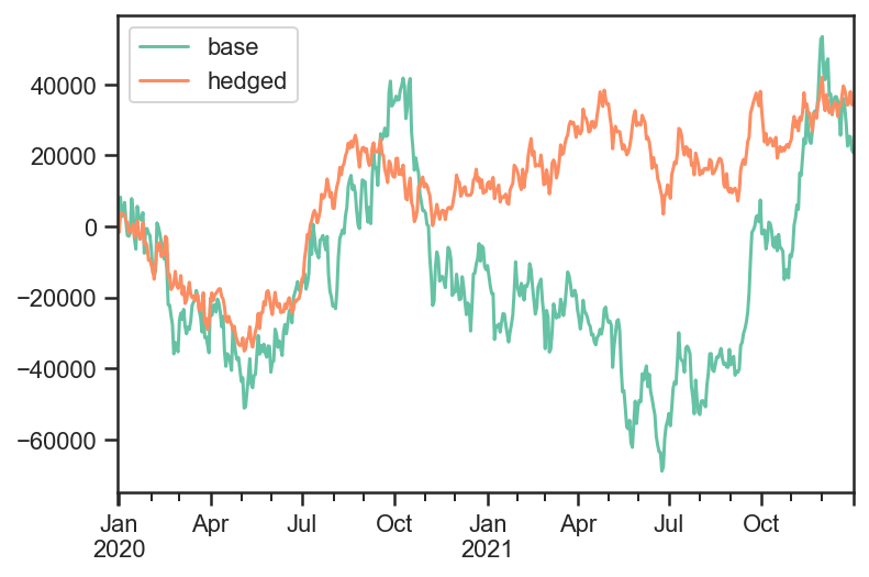
pd.DataFrame( {'base':base_test.strategy.values, 'hedged':hedge_test.strategy.values} ).plot();
# Total risk time series values
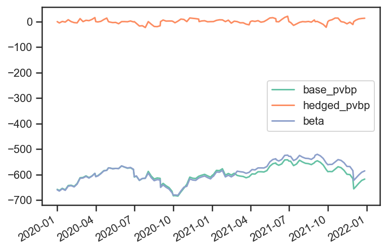
pd.DataFrame( {'base_pvbp':base_test.strategy.risks['pvbp'],
'hedged_pvbp':hedge_test.strategy.risks['pvbp'],
'beta':hedge_test.strategy.risks['beta']} ).dropna().plot();
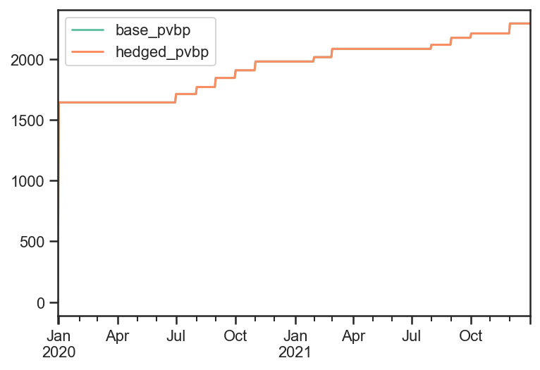
# Total bid/offer paid (same for both strategies)
pd.DataFrame( {'base_pvbp':base_test.strategy.bidoffers_paid,
               'hedged_pvbp':hedge_test.strategy.bidoffers_paid }).cumsum().dropna().plot();
Example 2: Nested Strategies
# Set up a more complex strategy and a backtest

# The goal of the more complex strategy is to define two sub-strategies of corporate bonds
# - Highest yield bonds
# - Lowest yield bonds
# Then we will go long the high yield bonds, short the low yield bonds in equal weight
# Lastly we will hedge the rates risk with the government bond

govt_securities = [ bt.CouponPayingHedgeSecurity( name ) for name in govt_data.index]
corp_securities = [ bt.CouponPayingSecurity( name ) for name in corp_data.index ]

def get_algos( n, sort_descending ):
    ''' Helper function to return the algos for long or short portfolio, based on top n yields'''
    return [
        # Close any matured bond positions
        bt.algos.ClosePositionsAfterDates( 'corp_maturity' ),
        # Specify how frequenty to rebalance
        bt.algos.RunMonthly(),
        # Select instruments for rebalancing. Start with everything
        bt.algos.SelectAll(),
        # Prevent matured/rolled instruments from coming back into the mix
        bt.algos.SelectActive(),
        # Set the stat to be used for selection
        bt.algos.SetStat( 'corp_yield' ),
        # Select the top N yielding bonds
        bt.algos.SelectN( n, sort_descending, filter_selected=True ),
        # Specify how to weigh the securities
        bt.algos.WeighEqually(),
        bt.algos.ScaleWeights(1. if sort_descending else -1.), # Determine long/short
        # Set the target portfolio size
        bt.algos.SetNotional( 'notional_value' ),
        # Rebalance the portfolio
        bt.algos.Rebalance(),
    ]
bottom_algos = []
top_strategy = bt.FixedIncomeStrategy('TopStrategy', get_algos( 10, True ), children = corp_securities)
bottom_strategy = bt.FixedIncomeStrategy('BottomStrategy',get_algos( 10, False ), children = corp_securities)

risk_stack = bt.AlgoStack(
    # Specify how frequently to calculate risk
    bt.algos.Or( [bt.algos.RunWeekly(),
                  bt.algos.RunMonthly()] ),
    # Update the risk given any positions that have been put on so far in the current step
    bt.algos.UpdateRisk( 'pvbp', history=2),
    bt.algos.UpdateRisk( 'beta', history=2),
)
hedging_stack = bt.AlgoStack(
    # Close any matured hedge positions (including hedges)
    bt.algos.ClosePositionsAfterDates( 'govt_maturity' ),
    # Roll government bond positions into the On The Run
    bt.algos.RollPositionsAfterDates( 'govt_roll_map' ),
    # Specify how frequently to hedge risk
    bt.algos.RunMonthly(),
    # Select the "alias" for the on-the-run government bond...
    bt.algos.SelectThese( [series_name], include_no_data = True ),
    # ... and then resolve it to the underlying security for the given date
    bt.algos.ResolveOnTheRun( 'govt_otr' ),
    # Hedge out the pvbp risk using the selected government bond
    bt.algos.HedgeRisks( ['pvbp']),
    # Need to update risk again after hedging so that it gets recorded correctly (post-hedges)
    bt.algos.UpdateRisk( 'pvbp', history=2),
)
debug_stack = bt.core.AlgoStack(
    # Specify how frequently to display debug info
    bt.algos.RunMonthly(),
    bt.algos.PrintInfo('{now}: End   {name}\tNotional:  {_notl_value:0.0f},\t Value: {_value:0.0f},\t Price: {_price:0.4f}'),
    bt.algos.PrintRisk('Risk: \tPVBP: {pvbp:0.0f},\t Beta: {beta:0.0f}'),
)
trading_stack =bt.core.AlgoStack(
    # Specify how frequently to rebalance the portfolio of sub-strategies
    bt.algos.RunOnce(),
    # Specify how to weigh the sub-strategies
    bt.algos.WeighSpecified( TopStrategy=0.5, BottomStrategy=-0.5),
    # Rebalance the portfolio
    bt.algos.Rebalance()
)

children = [ top_strategy, bottom_strategy ] + govt_securities
base_strategy = bt.FixedIncomeStrategy('BaseStrategy', [ bt.algos.Or( [trading_stack, risk_stack, debug_stack ] ) ], children = children)
hedged_strategy = bt.FixedIncomeStrategy('HedgedStrategy', [ bt.algos.Or( [trading_stack, risk_stack, hedging_stack, debug_stack ] ) ], children = children)

# Here we use clean prices as the data and accrued as the coupon. Could alternatively use dirty prices and cashflows.
data = pd.concat( [ govt_price, corp_price ], axis=1) / 100.  # Because we need prices per unit notional
additional_data = { 'coupons' : pd.concat([govt_accrued, corp_accrued], axis=1) / 100., # Because we need coupons per unit notional
                   'notional_value' : pd.Series( data=1e6, index=data.index ),
                   'govt_maturity' : govt_data.rename(columns={"mat_date": "date"}),
                   'corp_maturity' : corp_data.rename(columns={"mat_date": "date"}),
                   'govt_roll_map' : govt_roll_map,
                   'govt_otr' : govt_otr,
                   'corp_yield' : corp_yield,
                   'unit_risk' : {'pvbp' : pd.concat( [ govt_pvbp, corp_pvbp] ,axis=1)/100.,
                                  'beta' : corp_betas * corp_pvbp / 100.},
                  }
base_test = bt.Backtest( base_strategy, data, 'BaseBacktest',
                initial_capital = 0,
                additional_data = additional_data)
hedge_test = bt.Backtest( hedged_strategy, data, 'HedgedBacktest',
                initial_capital = 0,
                additional_data = additional_data)
out = bt.run( base_test, hedge_test )
 2020-01-01 00:00:00: End   BaseStrategy     Notional:  0,    Value: 0,       Price: 100.0000
 Risk:       PVBP: 0,         Beta: 0
 2020-02-03 00:00:00: End   BaseStrategy     Notional:  2000000,      Value: 3277,    Price: 100.1639
 Risk:       PVBP: 51,        Beta: 41
 2020-03-02 00:00:00: End   BaseStrategy     Notional:  2000000,      Value: 7297,    Price: 100.3649
 Risk:       PVBP: 45,        Beta: 34
 2020-04-01 00:00:00: End   BaseStrategy     Notional:  2000000,      Value: 9336,    Price: 100.4668
 Risk:       PVBP: 44,        Beta: 34
 2020-05-01 00:00:00: End   BaseStrategy     Notional:  2000000,      Value: 13453,   Price: 100.6727
 Risk:       PVBP: 38,        Beta: 28
 2020-06-01 00:00:00: End   BaseStrategy     Notional:  2000000,      Value: 15887,   Price: 100.7943
 Risk:       PVBP: 37,        Beta: 26
 2020-07-01 00:00:00: End   BaseStrategy     Notional:  1800000,      Value: 16024,   Price: 100.8010
 Risk:       PVBP: 39,        Beta: 28
 2020-08-03 00:00:00: End   BaseStrategy     Notional:  2000000,      Value: 14785,   Price: 100.7391
 Risk:       PVBP: -152,      Beta: -124
 2020-09-01 00:00:00: End   BaseStrategy     Notional:  1800000,      Value: 30310,   Price: 101.5550
 Risk:       PVBP: -263,      Beta: -204
 2020-10-01 00:00:00: End   BaseStrategy     Notional:  1900000,      Value: 35915,   Price: 101.8430
 Risk:       PVBP: -109,      Beta: -53
 2020-11-02 00:00:00: End   BaseStrategy     Notional:  2000000,      Value: 37649,   Price: 101.9297
 Risk:       PVBP: -12,       Beta: 36
 2020-12-01 00:00:00: End   BaseStrategy     Notional:  2000000,      Value: 39045,   Price: 101.9995
 Risk:       PVBP: -13,       Beta: 34
 2021-01-01 00:00:00: End   BaseStrategy     Notional:  2000000,      Value: 40569,   Price: 102.0758
 Risk:       PVBP: -14,       Beta: 31
 2021-02-01 00:00:00: End   BaseStrategy     Notional:  1900000,      Value: 41228,   Price: 102.1094
 Risk:       PVBP: -16,       Beta: 27
 2021-03-01 00:00:00: End   BaseStrategy     Notional:  1900000,      Value: 38916,   Price: 101.9868
 Risk:       PVBP: -101,      Beta: -47
 2021-04-01 00:00:00: End   BaseStrategy     Notional:  2000000,      Value: 40755,   Price: 102.0788
 Risk:       PVBP: 9,         Beta: -31
 2021-05-03 00:00:00: End   BaseStrategy     Notional:  2000000,      Value: 43290,   Price: 102.2055
 Risk:       PVBP: -6,        Beta: -43
 2021-06-01 00:00:00: End   BaseStrategy     Notional:  2000000,      Value: 35947,   Price: 101.8384
 Risk:       PVBP: -235,      Beta: -91
 2021-07-01 00:00:00: End   BaseStrategy     Notional:  2000000,      Value: 35671,   Price: 101.8246
 Risk:       PVBP: -123,      Beta: -129
 2021-08-02 00:00:00: End   BaseStrategy     Notional:  2000000,      Value: 37756,   Price: 101.9288
 Risk:       PVBP: 3,         Beta: -29
 2021-09-01 00:00:00: End   BaseStrategy     Notional:  2000000,      Value: 38434,   Price: 101.9627
 Risk:       PVBP: -7,        Beta: -43
 2021-10-01 00:00:00: End   BaseStrategy     Notional:  1900000,      Value: 37082,   Price: 101.8966
 Risk:       PVBP: 73,        Beta: 19
 2021-11-01 00:00:00: End   BaseStrategy     Notional:  2000000,      Value: 39526,   Price: 102.0187
 Risk:       PVBP: 51,        Beta: 53
 2021-12-01 00:00:00: End   BaseStrategy     Notional:  1900000,      Value: 29228,   Price: 101.4826
 Risk:       PVBP: 125,       Beta: 97
 2020-01-01 00:00:00: End   HedgedStrategy   Notional:  0,    Value: 0,       Price: 100.0000
 Risk:       PVBP: 0,         Beta: 0
 2020-02-03 00:00:00: End   HedgedStrategy   Notional:  2000000,      Value: 3277,    Price: 100.1639
 Risk:       PVBP: 0,         Beta: 41
 2020-03-02 00:00:00: End   HedgedStrategy   Notional:  2000000,      Value: 6159,    Price: 100.3079
 Risk:       PVBP: 0,         Beta: 34
 2020-04-01 00:00:00: End   HedgedStrategy   Notional:  2000000,      Value: 9008,    Price: 100.4504
 Risk:       PVBP: 0,         Beta: 34
 2020-05-01 00:00:00: End   HedgedStrategy   Notional:  2000000,      Value: 12274,   Price: 100.6137
 Risk:       PVBP: 0,         Beta: 28
 2020-06-01 00:00:00: End   HedgedStrategy   Notional:  2000000,      Value: 14189,   Price: 100.7094
 Risk:       PVBP: 0,         Beta: 26
 2020-07-01 00:00:00: End   HedgedStrategy   Notional:  1800000,      Value: 15451,   Price: 100.7752
 Risk:       PVBP: 0,         Beta: 28
 2020-08-03 00:00:00: End   HedgedStrategy   Notional:  2000000,      Value: 12494,   Price: 100.6273
 Risk:       PVBP: 0,         Beta: -124
 2020-09-01 00:00:00: End   HedgedStrategy   Notional:  1800000,      Value: 23384,   Price: 101.1967
 Risk:       PVBP: 0,         Beta: -204
 2020-10-01 00:00:00: End   HedgedStrategy   Notional:  1900000,      Value: 16414,   Price: 100.8372
 Risk:       PVBP: -0,        Beta: -53
 2020-11-02 00:00:00: End   HedgedStrategy   Notional:  2000000,      Value: 22887,   Price: 101.1609
 Risk:       PVBP: 0,         Beta: 36
 2020-12-01 00:00:00: End   HedgedStrategy   Notional:  2000000,      Value: 24681,   Price: 101.2506
 Risk:       PVBP: 0,         Beta: 34
 2021-01-01 00:00:00: End   HedgedStrategy   Notional:  2000000,      Value: 26080,   Price: 101.3205
 Risk:       PVBP: -0,        Beta: 31
 2021-02-01 00:00:00: End   HedgedStrategy   Notional:  1900000,      Value: 26954,   Price: 101.3647
 Risk:       PVBP: 0,         Beta: 27
 2021-03-01 00:00:00: End   HedgedStrategy   Notional:  1900000,      Value: 25008,   Price: 101.2611
 Risk:       PVBP: 0,         Beta: -47
 2021-04-01 00:00:00: End   HedgedStrategy   Notional:  2000000,      Value: 27730,   Price: 101.3972
 Risk:       PVBP: 0,         Beta: -31
 2021-05-03 00:00:00: End   HedgedStrategy   Notional:  2000000,      Value: 30112,   Price: 101.5163
 Risk:       PVBP: 0,         Beta: -43
 2021-06-01 00:00:00: End   HedgedStrategy   Notional:  2000000,      Value: 22951,   Price: 101.1582
 Risk:       PVBP: -0,        Beta: -91
 2021-07-01 00:00:00: End   HedgedStrategy   Notional:  2000000,      Value: 15553,   Price: 100.7884
 Risk:       PVBP: 0,         Beta: -129
 2021-08-02 00:00:00: End   HedgedStrategy   Notional:  2000000,      Value: 18657,   Price: 100.9436
 Risk:       PVBP: 0,         Beta: -29
 2021-09-01 00:00:00: End   HedgedStrategy   Notional:  2000000,      Value: 19441,   Price: 100.9827
 Risk:       PVBP: 0,         Beta: -43
 2021-10-01 00:00:00: End   HedgedStrategy   Notional:  1900000,      Value: 17903,   Price: 100.9072
 Risk:       PVBP: 0,         Beta: 19
 2021-11-01 00:00:00: End   HedgedStrategy   Notional:  2000000,      Value: 20524,   Price: 101.0383
 Risk:       PVBP: 0,         Beta: 53
 2021-12-01 00:00:00: End   HedgedStrategy   Notional:  1900000,      Value: 14170,   Price: 100.7071
 Risk:       PVBP: 0,         Beta: 97
# Total PNL time series values
pd.DataFrame( {'base':base_test.strategy.values,
               'hedged':hedge_test.strategy.values,
               'top':base_test.strategy['TopStrategy'].values,
               'bottom':base_test.strategy['BottomStrategy'].values}
            ).plot();
# Total pvbp time series values
pd.DataFrame( {'base':base_test.strategy.risks['pvbp'],
               'hedged':hedge_test.strategy.risks['pvbp'],
               'top':base_test.strategy['TopStrategy'].risks['pvbp'],
               'bottom':base_test.strategy['BottomStrategy'].risks['pvbp']}
            ).dropna().plot();
# Total beta time series values
pd.DataFrame( {'base':base_test.strategy.risks['beta'],
               'hedged':hedge_test.strategy.risks['beta'],
               'top':base_test.strategy['TopStrategy'].risks['beta'],
               'bottom':base_test.strategy['BottomStrategy'].risks['beta']}
            ).dropna().plot();
# "Price" time series values
pd.DataFrame( {'base':base_test.strategy.prices,
               'hedged':hedge_test.strategy.prices,
               'top':base_test.strategy['TopStrategy'].prices,
               'bottom':base_test.strategy['BottomStrategy'].prices}
            ).plot();
# Show transactions
out.get_transactions('HedgedBacktest').head(20)
| price | quantity | ||
|---|---|---|---|
| Date | Security | ||
| 2020-01-01 | corp0000 | 1.009697 | -100000.0 |
| corp0001 | 0.991417 | 100000.0 | |
| corp0002 | 1.016553 | -100000.0 | |
| corp0005 | 1.035779 | -100000.0 | |
| corp0009 | 1.014195 | 100000.0 | |
| corp0015 | 0.849097 | 100000.0 | |
| corp0017 | 1.018107 | -100000.0 | |
| corp0018 | 1.009549 | 100000.0 | |
| corp0019 | 0.908531 | 100000.0 | |
| corp0023 | 1.216847 | 100000.0 | |
| corp0024 | 1.094375 | -100000.0 | |
| corp0025 | 1.054762 | -100000.0 | |
| corp0030 | 0.888091 | 100000.0 | |
| corp0032 | 1.086487 | -100000.0 | |
| corp0035 | 0.996676 | 100000.0 | |
| corp0036 | 1.070212 | -100000.0 | |
| corp0037 | 0.992530 | 100000.0 | |
| corp0044 | 0.959150 | 100000.0 | |
| corp0048 | 0.987408 | -100000.0 | |
| corp0049 | 1.016879 | -100000.0 |